SUMMARY
- pheatmap() is useful for easy and pretty heatmap
- Demonstration of example() and demo() function
- How to reorder columns?
- How to add annotation bar with custom colors.
example(pheatmap)
##
## phetmp> # Create test matrix
## phetmp> test = matrix(rnorm(200), 20, 10)
##
## phetmp> test[1:10, seq(1, 10, 2)] = test[1:10, seq(1, 10, 2)] + 3
##
## phetmp> test[11:20, seq(2, 10, 2)] = test[11:20, seq(2, 10, 2)] + 2
##
## phetmp> test[15:20, seq(2, 10, 2)] = test[15:20, seq(2, 10, 2)] + 4
##
## phetmp> colnames(test) = paste("Test", 1:10, sep = "")
##
## phetmp> rownames(test) = paste("Gene", 1:20, sep = "")
##
## phetmp> # Draw heatmaps
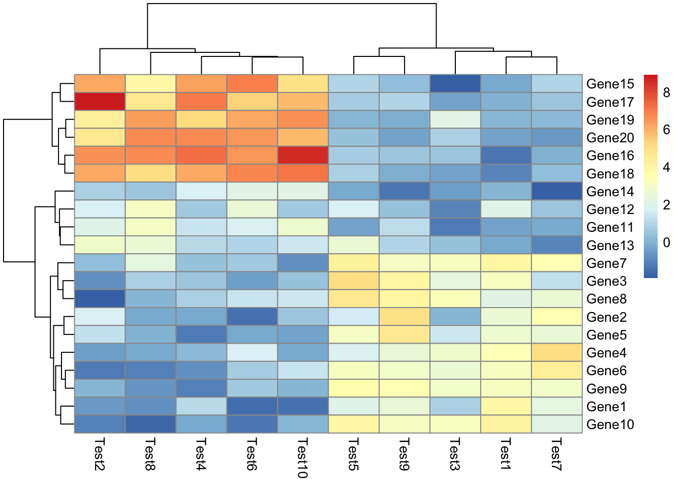
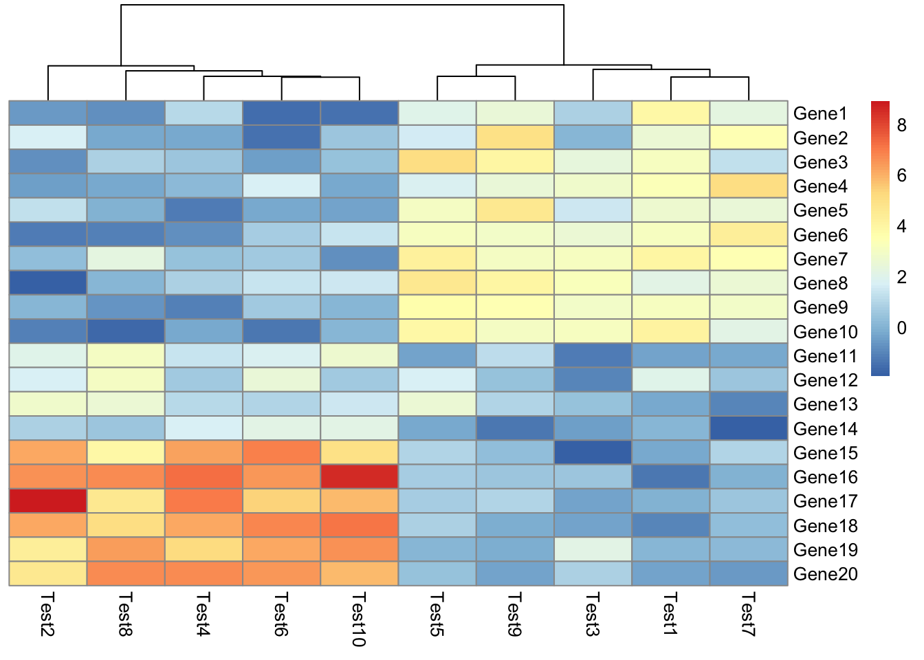
## phetmp> pheatmap(test)
##
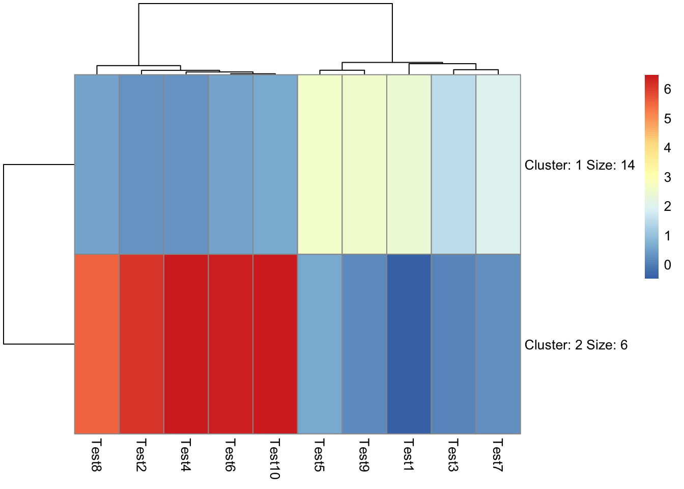
## phetmp> pheatmap(test, kmeans_k = 2)
##
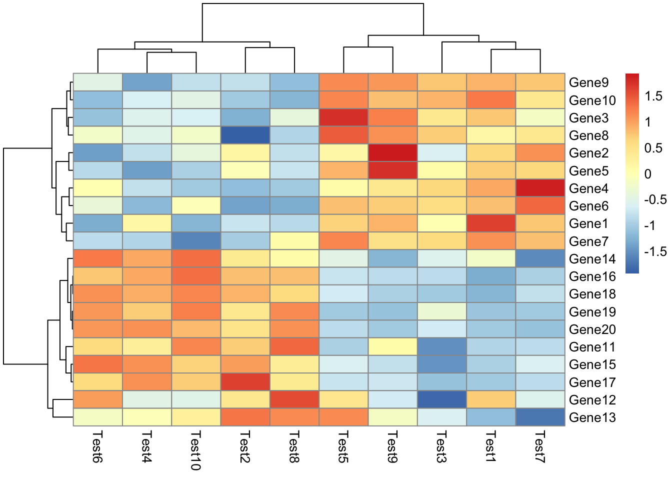
## phetmp> pheatmap(test, scale = "row", clustering_distance_rows = "correlation")
##
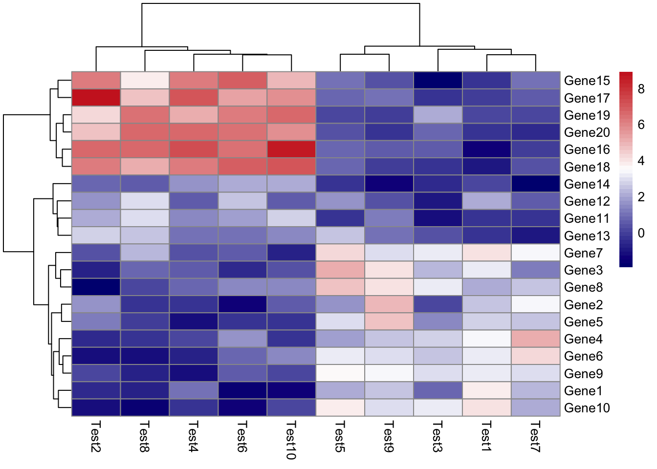
## phetmp> pheatmap(test, color = colorRampPalette(c("navy", "white", "firebrick3"))(50))
##
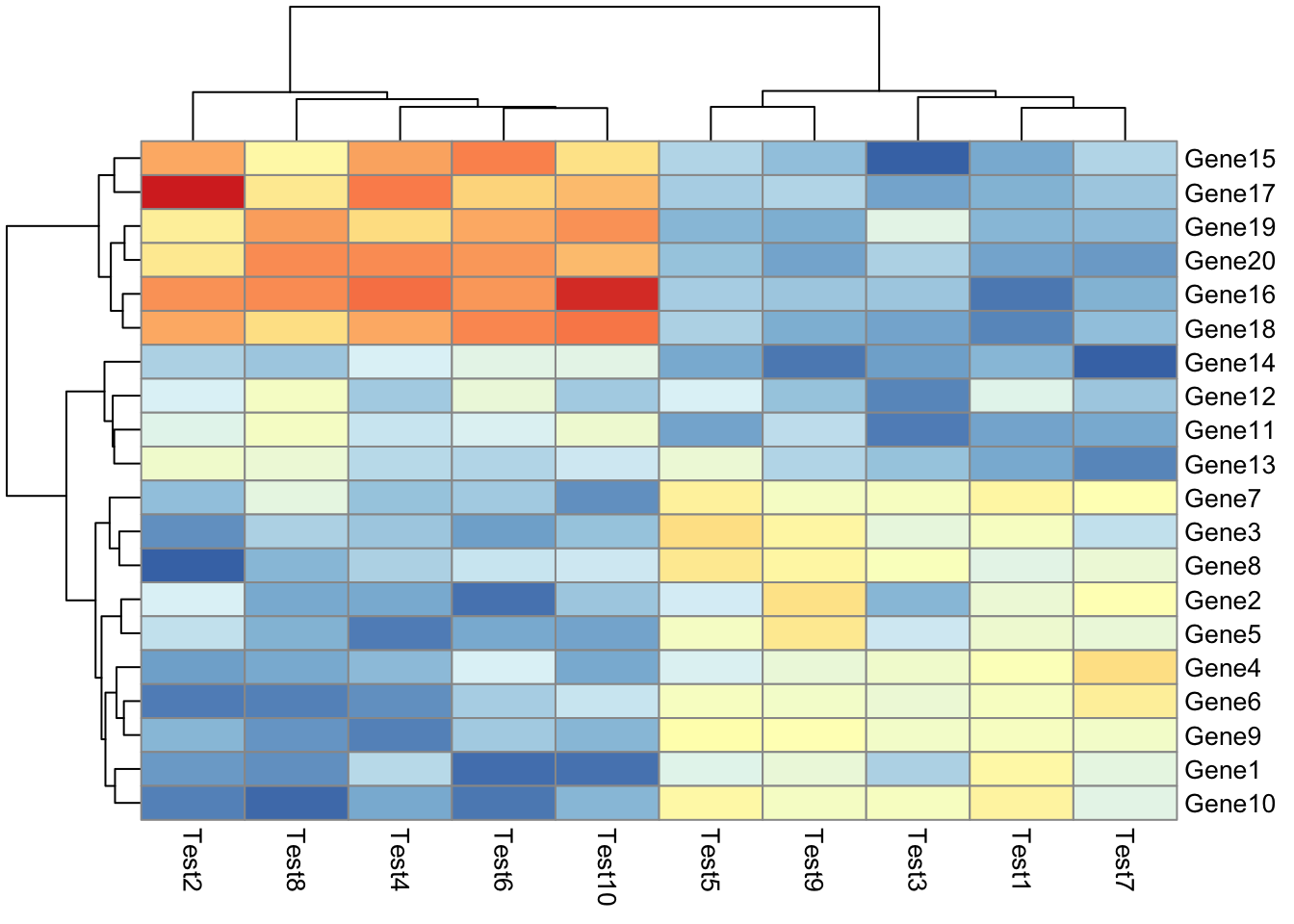
## phetmp> pheatmap(test, cluster_row = FALSE)
##
## phetmp> pheatmap(test, legend = FALSE)
##
## phetmp> # Show text within cells
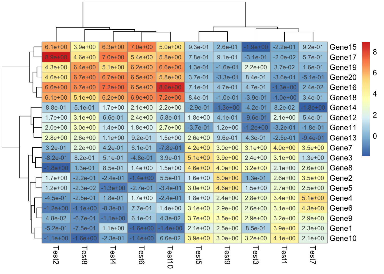
## phetmp> pheatmap(test, display_numbers = TRUE)

##
## phetmp> pheatmap(test, display_numbers = TRUE, number_format = "%.1e")
##
## phetmp> pheatmap(test, display_numbers = matrix(ifelse(test > 5, "*", ""), nrow(test)))

##
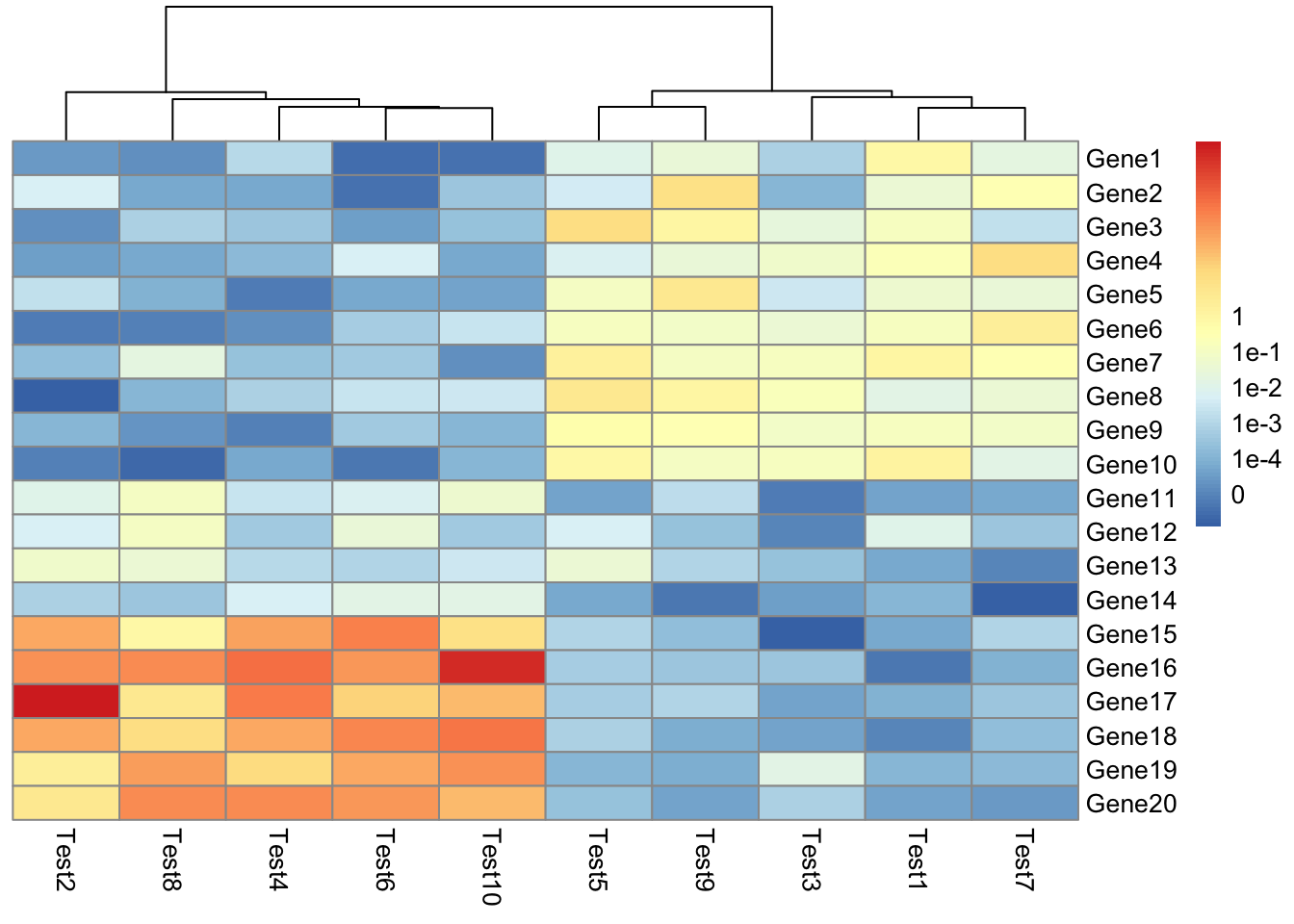
## phetmp> pheatmap(test, cluster_row = FALSE, legend_breaks = -1:4, legend_labels = c("0",
## phetmp+ "1e-4", "1e-3", "1e-2", "1e-1", "1"))
##
## phetmp> # Fix cell sizes and save to file with correct size
## phetmp> pheatmap(test, cellwidth = 15, cellheight = 12, main = "Example heatmap")
##
## phetmp> pheatmap(test, cellwidth = 15, cellheight = 12, fontsize = 8, filename = "test.pdf")
##
## phetmp> # Generate annotations for rows and columns
## phetmp> annotation_col = data.frame(
## phetmp+                     CellType = factor(rep(c("CT1", "CT2"), 5)),
## phetmp+                     Time = 1:5
## phetmp+                 )
##
## phetmp> rownames(annotation_col) = paste("Test", 1:10, sep = "")
##
## phetmp> annotation_row = data.frame(
## phetmp+                     GeneClass = factor(rep(c("Path1", "Path2", "Path3"), c(10, 4, 6)))
## phetmp+                 )
##
## phetmp> rownames(annotation_row) = paste("Gene", 1:20, sep = "")
##
## phetmp> # Display row and color annotations
## phetmp> pheatmap(test, annotation_col = annotation_col)
##
## phetmp> pheatmap(test, annotation_col = annotation_col, annotation_legend = FALSE)
##
## phetmp> pheatmap(test, annotation_col = annotation_col, annotation_row = annotation_row)
##
## phetmp> # Change angle of text in the columns
## phetmp> pheatmap(test, annotation_col = annotation_col, annotation_row = annotation_row, angle_col = "45")
##
## phetmp> pheatmap(test, annotation_col = annotation_col, angle_col = "0")
##
## phetmp> # Specify colors
## phetmp> ann_colors = list(
## phetmp+     Time = c("white", "firebrick"),
## phetmp+     CellType = c(CT1 = "#1B9E77", CT2 = "#D95F02"),
## phetmp+     GeneClass = c(Path1 = "#7570B3", Path2 = "#E7298A", Path3 = "#66A61E")
## phetmp+ )
##
## phetmp> pheatmap(test, annotation_col = annotation_col, annotation_colors = ann_colors, main = "Title")
##
## phetmp> pheatmap(test, annotation_col = annotation_col, annotation_row = annotation_row,
## phetmp+          annotation_colors = ann_colors)
##
## phetmp> pheatmap(test, annotation_col = annotation_col, annotation_colors = ann_colors[2])
##
## phetmp> # Gaps in heatmaps
## phetmp> pheatmap(test, annotation_col = annotation_col, cluster_rows = FALSE, gaps_row = c(10, 14))
##
## phetmp> pheatmap(test, annotation_col = annotation_col, cluster_rows = FALSE, gaps_row = c(10, 14),
## phetmp+          cutree_col = 2)
##
## phetmp> # Show custom strings as row/col names
## phetmp> labels_row = c("", "", "", "", "", "", "", "", "", "", "", "", "", "", "",
## phetmp+ "", "", "Il10", "Il15", "Il1b")
##
## phetmp> pheatmap(test, annotation_col = annotation_col, labels_row = labels_row)
##
## phetmp> # Specifying clustering from distance matrix
## phetmp> drows = dist(test, method = "minkowski")
##
## phetmp> dcols = dist(t(test), method = "minkowski")
##
## phetmp> pheatmap(test, clustering_distance_rows = drows, clustering_distance_cols = dcols)
##
## phetmp> # Modify ordering of the clusters using clustering callback option
## phetmp> callback = function(hc, mat){
## phetmp+     sv = svd(t(mat))$v[,1]
## phetmp+     dend = reorder(as.dendrogram(hc), wts = sv)
## phetmp+     as.hclust(dend)
## phetmp+ }
##
## phetmp> pheatmap(test, clustering_callback = callback)
##
## phetmp> ## Not run:
## phetmp> ##D # Same using dendsort package
## phetmp> ##D library(dendsort)
## phetmp> ##D
## phetmp> ##D callback = function(hc, ...){dendsort(hc)}
## phetmp> ##D pheatmap(test, clustering_callback = callback)
## phetmp> ## End(Not run)
## phetmp>
## phetmp>
## phetmp>
## phetmp>
demo()
demo(lm.glm, package = "stats", ask = TRUE)
##
##
## demo(lm.glm)
## ---- ~~~~~~
##
## > ### Examples from: "An Introduction to Statistical Modelling"
## > ### By Annette Dobson
## > ###
## > ### == with some additions ==
## >
## > # Copyright (C) 1997-2015 The R Core Team
## >
## > require(stats); require(graphics)
##
## > ## Plant Weight Data (Page 9)
## > ctl <- c(4.17,5.58,5.18,6.11,4.50,4.61,5.17,4.53,5.33,5.14)
##
## > trt <- c(4.81,4.17,4.41,3.59,5.87,3.83,6.03,4.89,4.32,4.69)
##
## > group <- gl(2,10, labels=c("Ctl","Trt"))
##
## > weight <- c(ctl,trt)
##
## > anova (lm(weight~group))
## Analysis of Variance Table
##
## Response: weight
## Df Sum Sq Mean Sq F value Pr(>F)
## group 1 0.6882 0.68820 1.4191 0.249
## Residuals 18 8.7293 0.48496
##
## > summary(lm(weight~group -1))
##
## Call:
## lm(formula = weight ~ group - 1)
##
## Residuals:
## Min 1Q Median 3Q Max
## -1.0710 -0.4938 0.0685 0.2462 1.3690
##
## Coefficients:
## Estimate Std. Error t value Pr(>|t|)
## groupCtl 5.0320 0.2202 22.85 9.55e-15 ***
## groupTrt 4.6610 0.2202 21.16 3.62e-14 ***
## ---
## Signif. codes: 0 '***' 0.001 '**' 0.01 '*' 0.05 '.' 0.1 ' ' 1
##
## Residual standard error: 0.6964 on 18 degrees of freedom
## Multiple R-squared: 0.9818, Adjusted R-squared: 0.9798
## F-statistic: 485.1 on 2 and 18 DF, p-value: < 2.2e-16
##
##
## > ## Birth Weight Data (Page 14)
## > age <- c(40, 38, 40, 35, 36, 37, 41, 40, 37, 38, 40, 38,
## + 40, 36, 40, 38, 42, 39, 40, 37, 36, 38, 39, 40)
##
## > birthw <- c(2968, 2795, 3163, 2925, 2625, 2847, 3292, 3473, 2628, 3176,
## + 3421, 2975, 3317, 2729, 2935, 2754, 3210, 2817, 3126, 2539,
## + 2412, 2991, 2875, 3231)
##
## > sex <- gl(2,12, labels=c("M","F"))
##
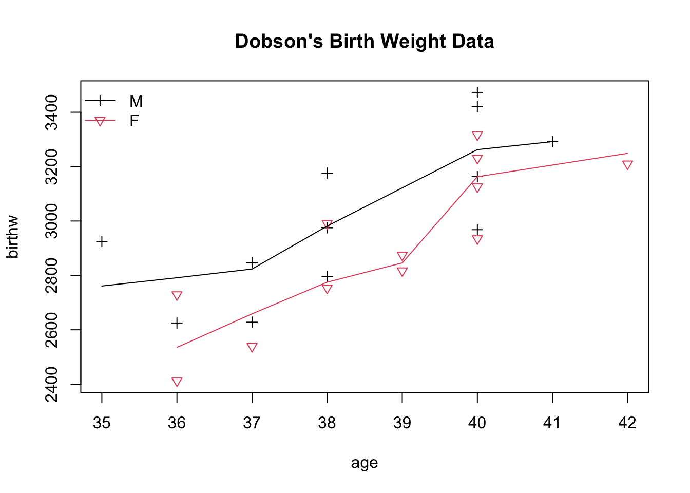
## > plot(age, birthw, col=as.numeric(sex), pch=3*as.numeric(sex),
## + main="Dobson's Birth Weight Data")
##
## > lines(lowess(age[sex=='M'], birthw[sex=='M']), col=1)
##
## > lines(lowess(age[sex=='F'], birthw[sex=='F']), col=2)
##
## > legend("topleft", levels(sex), col=1:2, pch=3*(1:2), lty=1, bty="n")
##
## > summary(l1 <- lm(birthw ~ sex + age), correlation=TRUE)
##
## Call:
## lm(formula = birthw ~ sex + age)
##
## Residuals:
## Min 1Q Median 3Q Max
## -257.49 -125.28 -58.44 169.00 303.98
##
## Coefficients:
## Estimate Std. Error t value Pr(>|t|)
## (Intercept) -1610.28 786.08 -2.049 0.0532 .
## sexF -163.04 72.81 -2.239 0.0361 *
## age 120.89 20.46 5.908 7.28e-06 ***
## ---
## Signif. codes: 0 '***' 0.001 '**' 0.01 '*' 0.05 '.' 0.1 ' ' 1
##
## Residual standard error: 177.1 on 21 degrees of freedom
## Multiple R-squared: 0.64, Adjusted R-squared: 0.6057
## F-statistic: 18.67 on 2 and 21 DF, p-value: 2.194e-05
##
## Correlation of Coefficients:
## (Intercept) sexF
## sexF 0.07
## age -1.00 -0.12
##
##
## > summary(l0 <- lm(birthw ~ sex + age -1), correlation=TRUE)
##
## Call:
## lm(formula = birthw ~ sex + age - 1)
##
## Residuals:
## Min 1Q Median 3Q Max
## -257.49 -125.28 -58.44 169.00 303.98
##
## Coefficients:
## Estimate Std. Error t value Pr(>|t|)
## sexM -1610.28 786.08 -2.049 0.0532 .
## sexF -1773.32 794.59 -2.232 0.0367 *
## age 120.89 20.46 5.908 7.28e-06 ***
## ---
## Signif. codes: 0 '***' 0.001 '**' 0.01 '*' 0.05 '.' 0.1 ' ' 1
##
## Residual standard error: 177.1 on 21 degrees of freedom
## Multiple R-squared: 0.9969, Adjusted R-squared: 0.9965
## F-statistic: 2258 on 3 and 21 DF, p-value: < 2.2e-16
##
## Correlation of Coefficients:
## sexM sexF
## sexF 1.00
## age -1.00 -1.00
##
##
## > anova(l1,l0)
## Analysis of Variance Table
##
## Model 1: birthw ~ sex + age
## Model 2: birthw ~ sex + age - 1
## Res.Df RSS Df Sum of Sq F Pr(>F)
## 1 21 658771
## 2 21 658771 0 -4.8894e-09
##
## > summary(li <- lm(birthw ~ sex + sex:age -1), correlation=TRUE)
##
## Call:
## lm(formula = birthw ~ sex + sex:age - 1)
##
## Residuals:
## Min 1Q Median 3Q Max
## -246.69 -138.11 -39.13 176.57 274.28
##
## Coefficients:
## Estimate Std. Error t value Pr(>|t|)
## sexM -1268.67 1114.64 -1.138 0.268492
## sexF -2141.67 1163.60 -1.841 0.080574 .
## sexM:age 111.98 29.05 3.855 0.000986 ***
## sexF:age 130.40 30.00 4.347 0.000313 ***
## ---
## Signif. codes: 0 '***' 0.001 '**' 0.01 '*' 0.05 '.' 0.1 ' ' 1
##
## Residual standard error: 180.6 on 20 degrees of freedom
## Multiple R-squared: 0.9969, Adjusted R-squared: 0.9963
## F-statistic: 1629 on 4 and 20 DF, p-value: < 2.2e-16
##
## Correlation of Coefficients:
## sexM sexF sexM:age
## sexF 0.00
## sexM:age -1.00 0.00
## sexF:age 0.00 -1.00 0.00
##
##
## > anova(li,l0)
## Analysis of Variance Table
##
## Model 1: birthw ~ sex + sex:age - 1
## Model 2: birthw ~ sex + age - 1
## Res.Df RSS Df Sum of Sq F Pr(>F)
## 1 20 652425
## 2 21 658771 -1 -6346.2 0.1945 0.6639
##
## > summary(zi <- glm(birthw ~ sex + age, family=gaussian()))
##
## Call:
## glm(formula = birthw ~ sex + age, family = gaussian())
##
## Coefficients:
## Estimate Std. Error t value Pr(>|t|)
## (Intercept) -1610.28 786.08 -2.049 0.0532 .
## sexF -163.04 72.81 -2.239 0.0361 *
## age 120.89 20.46 5.908 7.28e-06 ***
## ---
## Signif. codes: 0 '***' 0.001 '**' 0.01 '*' 0.05 '.' 0.1 ' ' 1
##
## (Dispersion parameter for gaussian family taken to be 31370.04)
##
## Null deviance: 1829873 on 23 degrees of freedom
## Residual deviance: 658771 on 21 degrees of freedom
## AIC: 321.39
##
## Number of Fisher Scoring iterations: 2
##
##
## > summary(z0 <- glm(birthw ~ sex + age - 1, family=gaussian()))
##
## Call:
## glm(formula = birthw ~ sex + age - 1, family = gaussian())
##
## Coefficients:
## Estimate Std. Error t value Pr(>|t|)
## sexM -1610.28 786.08 -2.049 0.0532 .
## sexF -1773.32 794.59 -2.232 0.0367 *
## age 120.89 20.46 5.908 7.28e-06 ***
## ---
## Signif. codes: 0 '***' 0.001 '**' 0.01 '*' 0.05 '.' 0.1 ' ' 1
##
## (Dispersion parameter for gaussian family taken to be 31370.04)
##
## Null deviance: 213198964 on 24 degrees of freedom
## Residual deviance: 658771 on 21 degrees of freedom
## AIC: 321.39
##
## Number of Fisher Scoring iterations: 2
##
##
## > anova(zi, z0)
## Analysis of Deviance Table
##
## Model 1: birthw ~ sex + age
## Model 2: birthw ~ sex + age - 1
## Resid. Df Resid. Dev Df Deviance F Pr(>F)
## 1 21 658771
## 2 21 658771 0 -2.3283e-10
##
## > summary(z.o4 <- update(z0, subset = -4))
##
## Call:
## glm(formula = birthw ~ sex + age - 1, family = gaussian(), subset = -4)
##
## Coefficients:
## Estimate Std. Error t value Pr(>|t|)
## sexM -2318.03 801.57 -2.892 0.00902 **
## sexF -2455.44 803.79 -3.055 0.00625 **
## age 138.50 20.71 6.688 1.65e-06 ***
## ---
## Signif. codes: 0 '***' 0.001 '**' 0.01 '*' 0.05 '.' 0.1 ' ' 1
##
## (Dispersion parameter for gaussian family taken to be 26925.39)
##
## Null deviance: 204643339 on 23 degrees of freedom
## Residual deviance: 538508 on 20 degrees of freedom
## AIC: 304.68
##
## Number of Fisher Scoring iterations: 2
##
##
## > summary(zz <- update(z0, birthw ~ sex+age-1 + sex:age))
##
## Call:
## glm(formula = birthw ~ sex + age + sex:age - 1, family = gaussian())
##
## Coefficients:
## Estimate Std. Error t value Pr(>|t|)
## sexM -1268.67 1114.64 -1.138 0.268492
## sexF -2141.67 1163.60 -1.841 0.080574 .
## age 111.98 29.05 3.855 0.000986 ***
## sexF:age 18.42 41.76 0.441 0.663893
## ---
## Signif. codes: 0 '***' 0.001 '**' 0.01 '*' 0.05 '.' 0.1 ' ' 1
##
## (Dispersion parameter for gaussian family taken to be 32621.23)
##
## Null deviance: 213198964 on 24 degrees of freedom
## Residual deviance: 652425 on 20 degrees of freedom
## AIC: 323.16
##
## Number of Fisher Scoring iterations: 2
##
##
## > anova(z0,zz)
## Analysis of Deviance Table
##
## Model 1: birthw ~ sex + age - 1
## Model 2: birthw ~ sex + age + sex:age - 1
## Resid. Df Resid. Dev Df Deviance F Pr(>F)
## 1 21 658771
## 2 20 652425 1 6346.2 0.1945 0.6639
##
## > ## Poisson Regression Data (Page 42)
## > x <- c(-1,-1,0,0,0,0,1,1,1)
##
## > y <- c(2,3,6,7,8,9,10,12,15)
##
## > summary(glm(y~x, family=poisson(link="identity")))
##
## Call:
## glm(formula = y ~ x, family = poisson(link = "identity"))
##
## Coefficients:
## Estimate Std. Error z value Pr(>|z|)
## (Intercept) 7.4516 0.8841 8.428 < 2e-16 ***
## x 4.9353 1.0892 4.531 5.86e-06 ***
## ---
## Signif. codes: 0 '***' 0.001 '**' 0.01 '*' 0.05 '.' 0.1 ' ' 1
##
## (Dispersion parameter for poisson family taken to be 1)
##
## Null deviance: 18.4206 on 8 degrees of freedom
## Residual deviance: 1.8947 on 7 degrees of freedom
## AIC: 40.008
##
## Number of Fisher Scoring iterations: 3
##
##
## > ## Calorie Data (Page 45)
## > calorie <- data.frame(
## + carb = c(33,40,37,27,30,43,34,48,30,38,
## + 50,51,30,36,41,42,46,24,35,37),
## + age = c(33,47,49,35,46,52,62,23,32,42,
## + 31,61,63,40,50,64,56,61,48,28),
## + wgt = c(100, 92,135,144,140,101, 95,101, 98,105,
## + 108, 85,130,127,109,107,117,100,118,102),
## + prot = c(14,15,18,12,15,15,14,17,15,14,
## + 17,19,19,20,15,16,18,13,18,14))
##
## > summary(lmcal <- lm(carb~age+wgt+prot, data= calorie))
##
## Call:
## lm(formula = carb ~ age + wgt + prot, data = calorie)
##
## Residuals:
## Min 1Q Median 3Q Max
## -10.3424 -4.8203 0.9897 3.8553 7.9087
##
## Coefficients:
## Estimate Std. Error t value Pr(>|t|)
## (Intercept) 36.96006 13.07128 2.828 0.01213 *
## age -0.11368 0.10933 -1.040 0.31389
## wgt -0.22802 0.08329 -2.738 0.01460 *
## prot 1.95771 0.63489 3.084 0.00712 **
## ---
## Signif. codes: 0 '***' 0.001 '**' 0.01 '*' 0.05 '.' 0.1 ' ' 1
##
## Residual standard error: 5.956 on 16 degrees of freedom
## Multiple R-squared: 0.4805, Adjusted R-squared: 0.3831
## F-statistic: 4.934 on 3 and 16 DF, p-value: 0.01297
##
##
## > ## Extended Plant Data (Page 59)
## > ctl <- c(4.17,5.58,5.18,6.11,4.50,4.61,5.17,4.53,5.33,5.14)
##
## > trtA <- c(4.81,4.17,4.41,3.59,5.87,3.83,6.03,4.89,4.32,4.69)
##
## > trtB <- c(6.31,5.12,5.54,5.50,5.37,5.29,4.92,6.15,5.80,5.26)
##
## > group <- gl(3, length(ctl), labels=c("Ctl","A","B"))
##
## > weight <- c(ctl,trtA,trtB)
##
## > anova(lmwg <- lm(weight~group))
## Analysis of Variance Table
##
## Response: weight
## Df Sum Sq Mean Sq F value Pr(>F)
## group 2 3.7663 1.8832 4.8461 0.01591 *
## Residuals 27 10.4921 0.3886
## ---
## Signif. codes: 0 '***' 0.001 '**' 0.01 '*' 0.05 '.' 0.1 ' ' 1
##
## > summary(lmwg)
##
## Call:
## lm(formula = weight ~ group)
##
## Residuals:
## Min 1Q Median 3Q Max
## -1.0710 -0.4180 -0.0060 0.2627 1.3690
##
## Coefficients:
## Estimate Std. Error t value Pr(>|t|)
## (Intercept) 5.0320 0.1971 25.527 <2e-16 ***
## groupA -0.3710 0.2788 -1.331 0.1944
## groupB 0.4940 0.2788 1.772 0.0877 .
## ---
## Signif. codes: 0 '***' 0.001 '**' 0.01 '*' 0.05 '.' 0.1 ' ' 1
##
## Residual standard error: 0.6234 on 27 degrees of freedom
## Multiple R-squared: 0.2641, Adjusted R-squared: 0.2096
## F-statistic: 4.846 on 2 and 27 DF, p-value: 0.01591
##
##
## > coef(lmwg)
## (Intercept) groupA groupB
## 5.032 -0.371 0.494
##
## > coef(summary(lmwg))#- incl. std.err, t- and P- values.
## Estimate Std. Error t value Pr(>|t|)
## (Intercept) 5.032 0.1971284 25.526514 1.936575e-20
## groupA -0.371 0.2787816 -1.330791 1.943879e-01
## groupB 0.494 0.2787816 1.771996 8.768168e-02
##
## > ## Fictitious Anova Data (Page 64)
## > y <- c(6.8,6.6,5.3,6.1,7.5,7.4,7.2,6.5,7.8,9.1,8.8,9.1)
##
## > a <- gl(3,4)
##
## > b <- gl(2,2, length(a))
##
## > anova(z <- lm(y~a*b))
## Analysis of Variance Table
##
## Response: y
## Df Sum Sq Mean Sq F value Pr(>F)
## a 2 12.7400 6.3700 25.8243 0.001127 **
## b 1 0.4033 0.4033 1.6351 0.248225
## a:b 2 1.2067 0.6033 2.4459 0.167164
## Residuals 6 1.4800 0.2467
## ---
## Signif. codes: 0 '***' 0.001 '**' 0.01 '*' 0.05 '.' 0.1 ' ' 1
##
## > ## Achievement Scores (Page 70)
## > y <- c(6,4,5,3,4,3,6, 8,9,7,9,8,5,7, 6,7,7,7,8,5,7)
##
## > x <- c(3,1,3,1,2,1,4, 4,5,5,4,3,1,2, 3,2,2,3,4,1,4)
##
## > m <- gl(3,7)
##
## > anova(z <- lm(y~x+m))
## Analysis of Variance Table
##
## Response: y
## Df Sum Sq Mean Sq F value Pr(>F)
## x 1 36.575 36.575 60.355 5.428e-07 ***
## m 2 16.932 8.466 13.970 0.0002579 ***
## Residuals 17 10.302 0.606
## ---
## Signif. codes: 0 '***' 0.001 '**' 0.01 '*' 0.05 '.' 0.1 ' ' 1
##
## > ## Beetle Data (Page 78)
## > dose <- c(1.6907, 1.7242, 1.7552, 1.7842, 1.8113, 1.8369, 1.861, 1.8839)
##
## > x <- c( 6, 13, 18, 28, 52, 53, 61, 60)
##
## > n <- c(59, 60, 62, 56, 63, 59, 62, 60)
##
## > dead <- cbind(x, n-x)
##
## > summary( glm(dead ~ dose, family=binomial(link=logit)))
##
## Call:
## glm(formula = dead ~ dose, family = binomial(link = logit))
##
## Coefficients:
## Estimate Std. Error z value Pr(>|z|)
## (Intercept) -60.717 5.181 -11.72 <2e-16 ***
## dose 34.270 2.912 11.77 <2e-16 ***
## ---
## Signif. codes: 0 '***' 0.001 '**' 0.01 '*' 0.05 '.' 0.1 ' ' 1
##
## (Dispersion parameter for binomial family taken to be 1)
##
## Null deviance: 284.202 on 7 degrees of freedom
## Residual deviance: 11.232 on 6 degrees of freedom
## AIC: 41.43
##
## Number of Fisher Scoring iterations: 4
##
##
## > summary( glm(dead ~ dose, family=binomial(link=probit)))
##
## Call:
## glm(formula = dead ~ dose, family = binomial(link = probit))
##
## Coefficients:
## Estimate Std. Error z value Pr(>|z|)
## (Intercept) -34.935 2.648 -13.19 <2e-16 ***
## dose 19.728 1.487 13.27 <2e-16 ***
## ---
## Signif. codes: 0 '***' 0.001 '**' 0.01 '*' 0.05 '.' 0.1 ' ' 1
##
## (Dispersion parameter for binomial family taken to be 1)
##
## Null deviance: 284.20 on 7 degrees of freedom
## Residual deviance: 10.12 on 6 degrees of freedom
## AIC: 40.318
##
## Number of Fisher Scoring iterations: 4
##
##
## > summary(z <- glm(dead ~ dose, family=binomial(link=cloglog)))
##
## Call:
## glm(formula = dead ~ dose, family = binomial(link = cloglog))
##
## Coefficients:
## Estimate Std. Error z value Pr(>|z|)
## (Intercept) -39.572 3.240 -12.21 <2e-16 ***
## dose 22.041 1.799 12.25 <2e-16 ***
## ---
## Signif. codes: 0 '***' 0.001 '**' 0.01 '*' 0.05 '.' 0.1 ' ' 1
##
## (Dispersion parameter for binomial family taken to be 1)
##
## Null deviance: 284.2024 on 7 degrees of freedom
## Residual deviance: 3.4464 on 6 degrees of freedom
## AIC: 33.644
##
## Number of Fisher Scoring iterations: 4
##
##
## > anova(z, update(z, dead ~ dose -1))
## Analysis of Deviance Table
##
## Model 1: dead ~ dose
## Model 2: dead ~ dose - 1
## Resid. Df Resid. Dev Df Deviance Pr(>Chi)
## 1 6 3.446
## 2 7 285.222 -1 -281.78 < 2.2e-16 ***
## ---
## Signif. codes: 0 '***' 0.001 '**' 0.01 '*' 0.05 '.' 0.1 ' ' 1
##
## > ## Anther Data (Page 84)
## > ## Note that the proportions below are not exactly
## > ## in accord with the sample sizes quoted below.
## > ## In particular, the last value, 5/9, should have been 0.556 instead of 0.555:
## > n <- c(102, 99, 108, 76, 81, 90)
##
## > p <- c(0.539,0.525,0.528,0.724,0.617,0.555)
##
## > x <- round(n*p)
##
## > ## x <- n*p
## > y <- cbind(x,n-x)
##
## > f <- rep(c(40,150,350),2)
##
## > (g <- gl(2,3))
## [1] 1 1 1 2 2 2
## Levels: 1 2
##
## > summary(glm(y ~ g*f, family=binomial(link="logit")))
##
## Call:
## glm(formula = y ~ g * f, family = binomial(link = "logit"))
##
## Coefficients:
## Estimate Std. Error z value Pr(>|z|)
## (Intercept) 0.1456719 0.1975451 0.737 0.4609
## g2 0.7963143 0.3125046 2.548 0.0108 *
## f -0.0001227 0.0008782 -0.140 0.8889
## g2:f -0.0020493 0.0013483 -1.520 0.1285
## ---
## Signif. codes: 0 '***' 0.001 '**' 0.01 '*' 0.05 '.' 0.1 ' ' 1
##
## (Dispersion parameter for binomial family taken to be 1)
##
## Null deviance: 10.45197 on 5 degrees of freedom
## Residual deviance: 0.60387 on 2 degrees of freedom
## AIC: 38.172
##
## Number of Fisher Scoring iterations: 3
##
##
## > summary(glm(y ~ g + f, family=binomial(link="logit")))
##
## Call:
## glm(formula = y ~ g + f, family = binomial(link = "logit"))
##
## Coefficients:
## Estimate Std. Error z value Pr(>|z|)
## (Intercept) 0.306643 0.167629 1.829 0.0674 .
## g2 0.405554 0.174560 2.323 0.0202 *
## f -0.000997 0.000665 -1.499 0.1338
## ---
## Signif. codes: 0 '***' 0.001 '**' 0.01 '*' 0.05 '.' 0.1 ' ' 1
##
## (Dispersion parameter for binomial family taken to be 1)
##
## Null deviance: 10.4520 on 5 degrees of freedom
## Residual deviance: 2.9218 on 3 degrees of freedom
## AIC: 38.49
##
## Number of Fisher Scoring iterations: 3
##
##
## > ## The "final model"
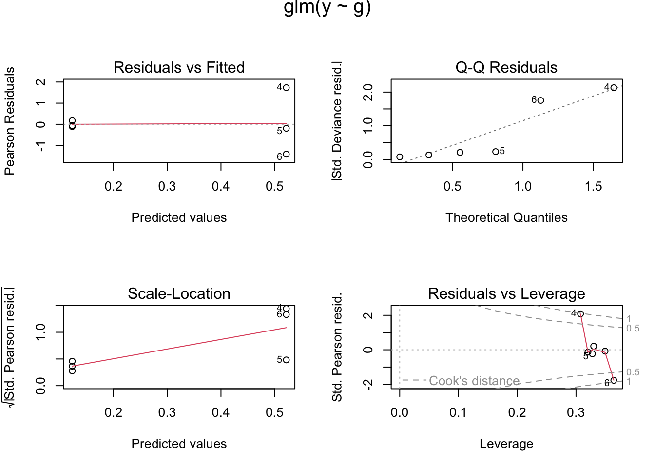
## > summary(glm.p84 <- glm(y~g, family=binomial(link="logit")))
##
## Call:
## glm(formula = y ~ g, family = binomial(link = "logit"))
##
## Coefficients:
## Estimate Std. Error z value Pr(>|z|)
## (Intercept) 0.1231 0.1140 1.080 0.2801
## g2 0.3985 0.1741 2.289 0.0221 *
## ---
## Signif. codes: 0 '***' 0.001 '**' 0.01 '*' 0.05 '.' 0.1 ' ' 1
##
## (Dispersion parameter for binomial family taken to be 1)
##
## Null deviance: 10.452 on 5 degrees of freedom
## Residual deviance: 5.173 on 4 degrees of freedom
## AIC: 38.741
##
## Number of Fisher Scoring iterations: 3
##
##
## > op <- par(mfrow = c(2,2), oma = c(0,0,1,0))
##
## > plot(glm.p84) # well ?
##
## > par(op)
##
## > ## Tumour Data (Page 92)
## > counts <- c(22,2,10,16,54,115,19,33,73,11,17,28)
##
## > type <- gl(4,3,12,labels=c("freckle","superficial","nodular","indeterminate"))
##
## > site <- gl(3,1,12,labels=c("head/neck","trunk","extremities"))
##
## > data.frame(counts,type,site)
##    counts          type        site
## 1      22       freckle   head/neck
## 2       2       freckle       trunk
## 3      10       freckle extremities
## 4      16   superficial   head/neck
## 5      54   superficial       trunk
## 6     115   superficial extremities
## 7      19       nodular   head/neck
## 8      33       nodular       trunk
## 9      73       nodular extremities
## 10     11 indeterminate   head/neck
## 11     17 indeterminate       trunk
## 12     28 indeterminate extremities
##
## > summary(z <- glm(counts ~ type + site, family=poisson()))
##
## Call:
## glm(formula = counts ~ type + site, family = poisson())
##
## Coefficients:
##                   Estimate Std. Error z value Pr(>|z|)
## (Intercept)         1.7544     0.2040   8.600  < 2e-16 ***
## typesuperficial     1.6940     0.1866   9.079  < 2e-16 ***
## typenodular         1.3020     0.1934   6.731 1.68e-11 ***
## typeindeterminate   0.4990     0.2174   2.295  0.02173 *
## sitetrunk           0.4439     0.1554   2.857  0.00427 **
## siteextremities     1.2010     0.1383   8.683  < 2e-16 ***
## ---
## Signif. codes:  0 '***' 0.001 '**' 0.01 '*' 0.05 '.' 0.1 ' ' 1
##
## (Dispersion parameter for poisson family taken to be 1)
##
##     Null deviance: 295.203  on 11  degrees of freedom
## Residual deviance:  51.795  on  6  degrees of freedom
## AIC: 122.91
##
## Number of Fisher Scoring iterations: 5
##
##
## > ## Randomized Controlled Trial (Page 93)
## > counts <- c(18,17,15, 20,10,20, 25,13,12)
##
## > outcome   <- gl(3, 1, length(counts))
##
## > treatment <- gl(3, 3)
##
## > summary(z <- glm(counts ~ outcome + treatment, family=poisson()))
##
## Call:
## glm(formula = counts ~ outcome + treatment, family = poisson())
##
## Coefficients:
##               Estimate Std. Error z value Pr(>|z|)
## (Intercept)  3.045e+00  1.709e-01  17.815   <2e-16 ***
## outcome2    -4.543e-01  2.022e-01  -2.247   0.0246 *
## outcome3    -2.930e-01  1.927e-01  -1.520   0.1285
## treatment2   1.398e-16  2.000e-01   0.000   1.0000
## treatment3  -2.416e-16  2.000e-01   0.000   1.0000
## ---
## Signif. codes:  0 '***' 0.001 '**' 0.01 '*' 0.05 '.' 0.1 ' ' 1
##
## (Dispersion parameter for poisson family taken to be 1)
##
##     Null deviance: 10.5814  on 8  degrees of freedom
## Residual deviance:  5.1291  on 4  degrees of freedom
## AIC: 56.761
##
## Number of Fisher Scoring iterations: 4
##
##
## > ## Peptic Ulcers and Blood Groups
## > counts <- c(579, 4219, 911, 4578, 246, 3775, 361, 4532, 291, 5261, 396, 6598)
##
## > group <- gl(2, 1, 12, labels=c("cases","controls"))
##
## > blood <- gl(2, 2, 12, labels=c("A","O"))
##
## > city  <- gl(3, 4, 12, labels=c("London","Manchester","Newcastle"))
##
## > cbind(group, blood, city, counts) # gives internal codes for the factors
##       group blood city counts
##  [1,]     1     1    1    579
##  [2,]     2     1    1   4219
##  [3,]     1     2    1    911
##  [4,]     2     2    1   4578
##  [5,]     1     1    2    246
##  [6,]     2     1    2   3775
##  [7,]     1     2    2    361
##  [8,]     2     2    2   4532
##  [9,]     1     1    3    291
## [10,]     2     1    3   5261
## [11,]     1     2    3    396
## [12,]     2     2    3   6598
##
## > summary(z1 <- glm(counts ~ group*(city + blood), family=poisson()))
##
## Call:
## glm(formula = counts ~ group * (city + blood), family = poisson())
##
## Coefficients:
##                              Estimate Std. Error z value Pr(>|z|)
## (Intercept)                   6.39239    0.03476  183.92  < 2e-16 ***
## groupcontrols                 1.90813    0.03691   51.69  < 2e-16 ***
## cityManchester               -0.89800    0.04815  -18.65  < 2e-16 ***
## cityNewcastle                -0.77420    0.04612  -16.79  < 2e-16 ***
## bloodO                        0.40187    0.03867   10.39  < 2e-16 ***
## groupcontrols:cityManchester  0.84069    0.05052   16.64  < 2e-16 ***
## groupcontrols:cityNewcastle   1.07287    0.04822   22.25  < 2e-16 ***
## groupcontrols:bloodO         -0.23208    0.04043   -5.74 9.46e-09 ***
## ---
## Signif. codes:  0 '***' 0.001 '**' 0.01 '*' 0.05 '.' 0.1 ' ' 1
##
## (Dispersion parameter for poisson family taken to be 1)
##
##     Null deviance: 26717.157  on 11  degrees of freedom
## Residual deviance:    29.241  on  4  degrees of freedom
## AIC: 154.32
##
## Number of Fisher Scoring iterations: 3
##
##
## > summary(z2 <- glm(counts ~ group*city + blood, family=poisson()),
## +         correlation = TRUE)
##
## Call:
## glm(formula = counts ~ group * city + blood, family = poisson())
##
## Coefficients:
##                              Estimate Std. Error z value Pr(>|z|)
## (Intercept)                   6.51395    0.02663  244.60   <2e-16 ***
## groupcontrols                 1.77563    0.02801   63.38   <2e-16 ***
## cityManchester               -0.89800    0.04815  -18.65   <2e-16 ***
## cityNewcastle                -0.77420    0.04612  -16.79   <2e-16 ***
## bloodO                        0.18988    0.01128   16.84   <2e-16 ***
## groupcontrols:cityManchester  0.84069    0.05052   16.64   <2e-16 ***
## groupcontrols:cityNewcastle   1.07287    0.04822   22.25   <2e-16 ***
## ---
## Signif. codes:  0 '***' 0.001 '**' 0.01 '*' 0.05 '.' 0.1 ' ' 1
##
## (Dispersion parameter for poisson family taken to be 1)
##
##     Null deviance: 26717.157  on 11  degrees of freedom
## Residual deviance:    62.558  on  5  degrees of freedom
## AIC: 185.63
##
## Number of Fisher Scoring iterations: 4
##
## Correlation of Coefficients:
##                              (Intercept) groupcontrols cityManchester
## groupcontrols                -0.90
## cityManchester               -0.52        0.50
## cityNewcastle                -0.55        0.52          0.30
## bloodO                       -0.23        0.00          0.00
## groupcontrols:cityManchester  0.50       -0.55         -0.95
## groupcontrols:cityNewcastle   0.52       -0.58         -0.29
##                              cityNewcastle bloodO groupcontrols:cityManchester
## groupcontrols
## cityManchester
## cityNewcastle
## bloodO                        0.00
## groupcontrols:cityManchester -0.29          0.00
## groupcontrols:cityNewcastle  -0.96          0.00   0.32
##
##
## > anova(z2, z1, test = "Chisq")
## Analysis of Deviance Table
##
## Model 1: counts ~ group * city + blood
## Model 2: counts ~ group * (city + blood)
##   Resid. Df Resid. Dev Df Deviance  Pr(>Chi)
## 1         5     62.558
## 2         4     29.241  1   33.318 7.827e-09 ***
## ---
## Signif. codes:  0 '***' 0.001 '**' 0.01 '*' 0.05 '.' 0.1 ' ' 1