Installing BioVizSeq package
struggle with package installation
#install.packages("BioVizSeq")
library(BioVizSeq)
#library(shinydashboard)
#install.packages("shinycssloaders") # /var/folders/_w/7dj610fh8xn6h8001s7_5h3r0000gn/T//Rtmph1L7Mw/downloaded_packages
#install.packages("shinycssloaders",lib="/var/folders/_w/7dj610fh8xn6h8001s7_5h3r0000gn/T//Rtmph1L7Mw/downloaded_packages/shinycssloaders")
#install.packages("/Users/nozue/Downloads/shinydashboard_0.7.3.tar.gz", repos = NULL, type = "source")
#library(shinycssloaders)
#library(shinyWidgets)
#biovizseq()
First get plant promoter motif search at PlantCARE site
This site is using plant promoter motif database. But the promoter motif data is old.
RAM1 (“Solyc02g094340.1”), RAM2 (“Solyc02g087500.3”, “Solyc04g005840.1”, “Solyc10g084900.1”)
library(BioVizSeq)## Package BioVizSeq loaded successfully!# SL RAM1 prom data (PlantCARE_16059), PlantCARE_16059_SL_RAM1prom_plantCARE
plantcare_file.Solyc02g094340 <- read.table("/Volumes/data_work/Data6/Sinha_lab/PlasticityIII_AMF_TRAP/AMF_responsive_gene_promoters/PlantCARE_16059_SL_RAM1_prom_plantCARE/plantCARE_output_PlantCARE_16059.tab", header = FALSE, sep = '\t', quote="")
# SL RAM2a (tentatively called) "Solyc02g087500.3" prom data ()
plantcare_file.Solyc02g087500 <- read.table("/Volumes/data_work/Data6/Sinha_lab/PlasticityIII_AMF_TRAP/AMF_responsive_gene_promoters/PlantCARE_18029_RAM2a_prom_plantCARE/plantCARE_output_PlantCARE_18029.tab", header = FALSE, sep = '\t', quote="")
# SL RAM2b prom data Solyc04g005840, PlantCARE_28616
plantcare_file.Solyc04g005840 <- read.table("/Volumes/data_work/Data6/Sinha_lab/PlasticityIII_AMF_TRAP/AMF_responsive_gene_promoters/PlantCARE_28616_SLRAM2B_prom_plantCARE/plantCARE_output_PlantCARE_28616.tab", header = FALSE, sep = '\t', quote="")
# SL RAM2c prom data Solyc10g084900 PlantCARE_31086
plantcare_file.Solyc10g08490 <- read.table("/Volumes/data_work/Data6/Sinha_lab/PlasticityIII_AMF_TRAP/AMF_responsive_gene_promoters/PlantCARE_31086_SLRAM2C_prom_plantCARE/plantCARE_output_PlantCARE_31086.tab", header = FALSE, sep = '\t', quote="")
# change format
plantcare_file.Solyc02g094340 <- plantcare_classify(plantcare_file.Solyc02g094340) %>% mutate(ID="RAM1 Solyc02g094340")
plantcare_file.Solyc02g087500 <- plantcare_classify(plantcare_file.Solyc02g087500) %>% mutate(ID="RAM2a Solyc02g087500")
plantcare_file.Solyc04g005840 <- plantcare_classify(plantcare_file.Solyc04g005840) %>% mutate(ID="RAM2b Solyc04g005840")
plantcare_file.Solyc10g08490 <- plantcare_classify(plantcare_file.Solyc10g08490) %>% mutate(ID="RAM2c Solyc10g08490")
# combine
plantcare_loc <- plantcare_to_loc(bind_rows(plantcare_file.Solyc02g094340,plantcare_file.Solyc02g087500, plantcare_file.Solyc04g005840, plantcare_file.Solyc10g08490))
promoter_length <- data.frame(ID = unique(plantcare_loc$ID), length=5000)
# all elements
motif_plot(plantcare_loc, promoter_length,show_motif_id=FALSE) + labs(x="Promoter Length", y="Gene")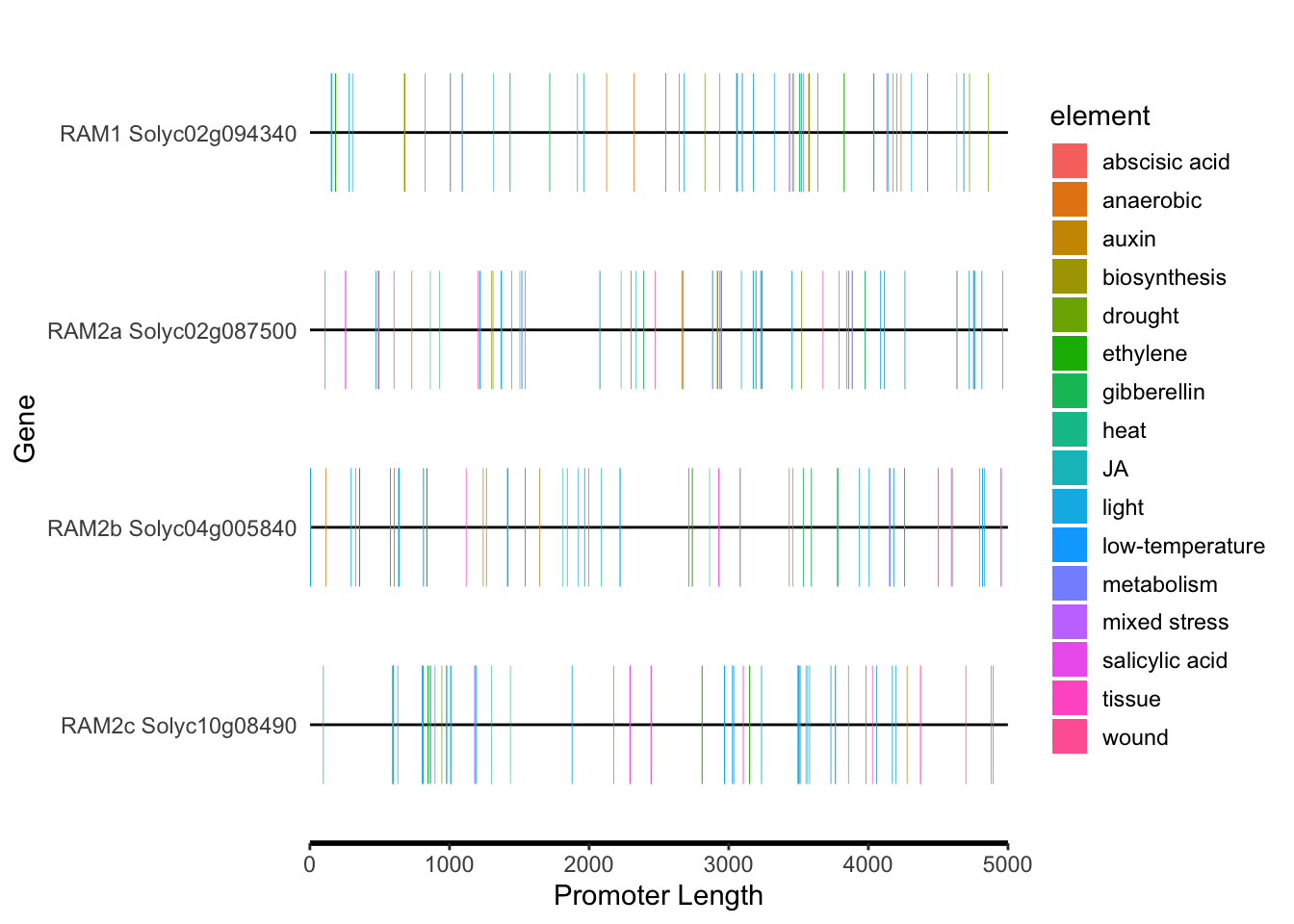
# "abscisic acid", SA, JA, mixed stress, wound, ethylene
motif_plot(plantcare_loc %>% dplyr::filter(Element %in% c("salicylic acid","JA","abscisic acid","mixed stress","wound","ethylene")), promoter_length,show_motif_id=FALSE) + labs(x="Promoter Length", y="Gene") 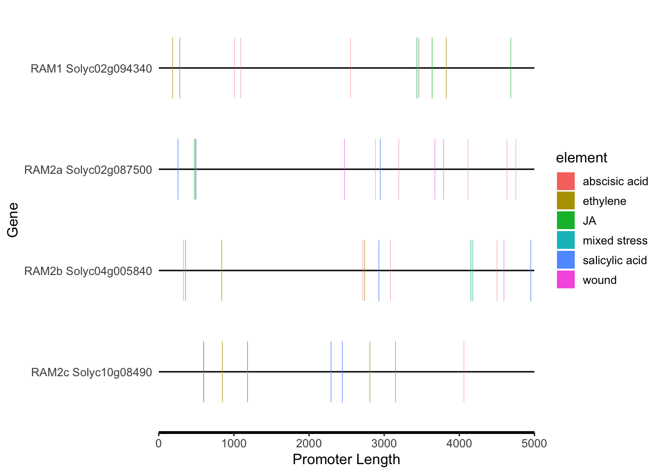
# facet_grid does not work
#motif_plot(plantcare_loc, promoter_length,show_motif_id=FALSE) + labs(x="Promoter Length", y="Gene") + facet_wrap(element~.)
# SA and JA
motif_plot(plantcare_loc  %>% dplyr::filter(Element %in% c("salicylic acid","JA")), promoter_length,show_motif_id=FALSE) + labs(x="Promoter Length", y="Gene")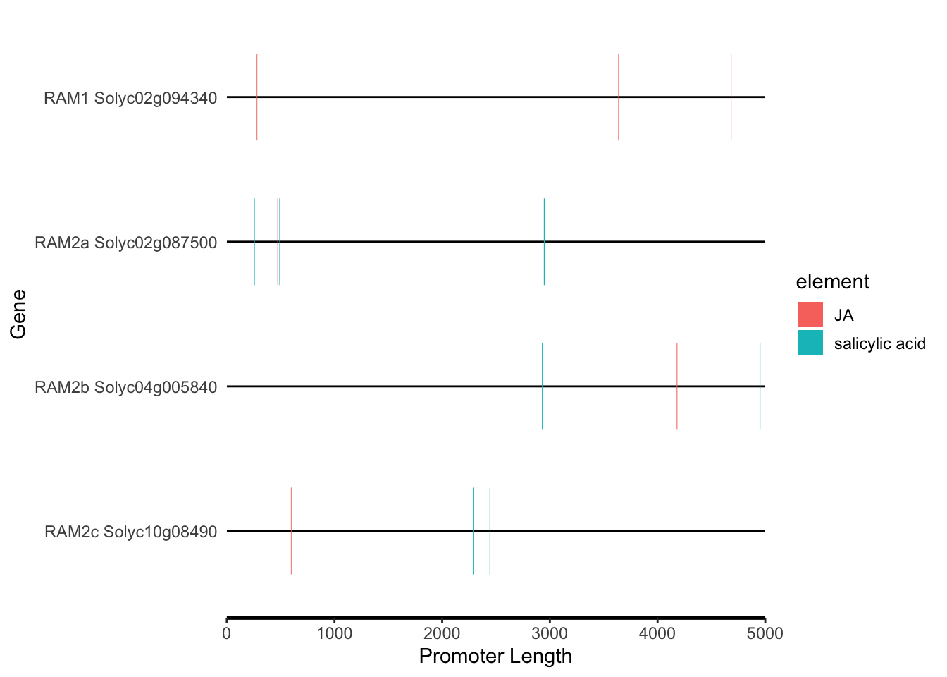
How to plot promoter motif of interest in FYI gene promoters (~ 100 genes)?
PHOSPHATE STARVATION RESPONSE (PHR) transcription factors belong to the MYB transcription factor (TF) family and bind to PHR1 binding site (P1BS) motifs (GNATATNC) in the promoters of phosphate starvation-induced (PSI) genes. Rice OsPHS2 is necessary for AMF colonization (Das 2022). Here I am just looking P1BS motifs in core AMF pathway genes in tomato reported in Zeng 2023.
step A. Bulk extraction of 2 kb promoter region sequences of all tomato genes.
step B. Get gene of interest (this thime, AMF core genes)
step C. Extract the promoter sequences of FYI genes in step B.
step D. Find a promoter motif of interest in the promoter sequences (in fasta format)
step E. Plot the position of the motif in the promoters
step A. extract promoters of genes of interest by bulk extraction of promoter sequences using EnsemblPlant BioMart interface
Step 1: Access the BioMart interface
Go to the Ensembl Plants website. Click on the BioMart link, which is usually located in the header or in the “Tools” section.
Step 2: Select the database and dataset
On the BioMart page, under “CHOOSE DATABASE,” select Ensembl Plants Genes. Under “CHOOSE DATASET,” find and select your species of interest (e.g., Arabidopsis thaliana genes or Zea mays genes).
Step 3: Add your gene filters
In the left-hand panel, click Filters. Expand the “GENE” section. Here you can input your gene list. For example, use the filter “Gene stable ID(s)” and paste a list of Ensembl gene IDs. You can use other filters, such as gene name or chromosome location, if you don’t have a list of Ensembl gene IDs.
Step 4: Define the sequence attributes
In the left-hand panel, click Attributes. Expand the “SEQUENCES” section. Select the “Flank (Upstream)” attribute. This is the crucial step for defining the promoter region. In the “Flank (Upstream)” options, specify the following: Upstream flanking region: Enter the number of base pairs you want to retrieve upstream of the gene’s transcription start site (e.g., 1500 bp, a common length for promoter analysis). Downstream flanking region: Set this to 0 since you only want the upstream region. Strand: Select “Coding strand” or “Sense strand”. For promoter extraction, retrieving the sequence on the same strand as the gene is standard.
Step 5: Configure your output
Under the “ATTRIBUTES” section, you can add other desired output information, such as “Gene stable ID” or “Associated Gene Name” to easily link the sequences back to your original genes. Click the “Results” button in the left-hand panel. On the results page, you can review a preview of your query. To download the sequences, click “Export all results to”. Select “File”, choose “FASTA” as the file format, and then click the “Go” button. This will download your promoter sequences in FASTA format.
Step B. Orthogroup table (supplementary table S7) for AMF core genes reported in Zeng 2023.
library(tidyverse)
Zeng_2023_S7 <- readxl::read_excel("/Volumes/data_work/Data6/Sinha_lab/PlasticityIII_AMF_TRAP/ScienceDirect_files_20Feb2024_21-27-28.124/1-s2.0-S2590346222002619-mmc2.xlsx",sheet="Table S7",skip=1) %>% drop_na()
# needs to format this table to use inner_join() (see "00_annotation.Rmd")

# step1 for itag4.1
brake.into.singleID4a <- function(DT=Zeng_2023_S7,target.column="Solanum_lycopersicum") {
  #target.column <- enquo(target.column)
  print(target.column)
  x <- DT %>% dplyr::select(all_of(target.column))  %>% as_vector() %>% str_split(", ") %>% unlist()
DT %>% dplyr::select(-all_of(target.column)) %>% right_join(tibble(Orthogroup=rep(DT %>% dplyr::select(Orthogroup) %>% as_vector(),length(x)), Solanum_lycopersicum = x))
}
# test
temp <- brake.into.singleID4a(DT=Zeng_2023_S7 %>% dplyr::slice(1:1))
#
for(n in 1:dim(Zeng_2023_S7)[1]) {
  print("n is ");print(n)
temp <- temp %>% bind_rows(brake.into.singleID4a(Zeng_2023_S7 %>% dplyr::slice(n:n)))
}
temp %>% View()
Zeng_2023_S7.v2 <- temp %>% separate(Solanum_lycopersicum,sep="\\.",into="gene",extra="drop",fill="left",remove=FALSE)
Zeng_2023_S7.v2 %>% View()
# extract only tomato genes and format
SL.AMFcore.Zeng2023.gene.df <- Zeng_2023_S7.v2 %>% distinct(Solanum_lycopersicum) %>% dplyr::select(Solanum_lycopersicum) %>% mutate(Solanum_lycopersicum=str_remove_all(Solanum_lycopersicum,"Sly_")) %>% separate(Solanum_lycopersicum,c("v1","v2","v3"),remove=FALSE) %>% filter(str_detect(Solanum_lycopersicum,"Solyc")) %>% select(v1)
# write
write_csv(SL.AMFcore.Zeng2023.gene.df,file.path("SL.AMFcore.Zeng2023.gene.csv"))
#
SL.AMFcore.Zeng2023.gene <- SL.AMFcore.Zeng2023.gene.df %>% as_vector()
Step C-1 modify output from Biomart in EnesmbplePlant by awk in UNIX
system("awk '/^>/ {if (N>0) printf(\"\\n\"); printf(\"%s\\t\",$0); N++; next;} {printf(\"%s\",$0);} END {printf(\"\\n\");}' mart_export.txt > mart_export_mod.txt")
# look
system("head mart_export_mod.txt")
Step C-2 Extracting promoter sequences of FYI genes by R + UNIX. Learning from ChatGPT answer.
out_file <- "SL.AMFcore.Zeng2023_prom2000.fasta"
# shQuote() is for Quote a string to be passed to an operating system shell.
for (gene in SL.AMFcore.Zeng2023.gene) {
  cmd <- paste(
    "grep", shQuote(gene),
    "mart_export_mod.txt | tr '\\t' '\\n' >>", out_file
  )
  print(cmd)
  system(cmd) # run UNIX command
} # works well
Step D. PIBS promoter motif analysis
Custom motif (“GNATATNC” for P1BS) finding in given promoter sequences “RSAT - dna-pattern” used in Das (2022).
Step E. read P1BS promoter motif analysis resuls RSAT website and plot
Use BioVizSeq package above.
library(BioVizSeq)
# remove ";" for column name
SL.AMFcore.Zeng2023.P1BS <- readr::read_delim(file.path("/Volumes","data_work","Data8","NGS_related","Sinha_lab","RNAseq_tomato_AMF","output","dna-pattern_2025-08-28.072501_h5Ildx.pat"), comment=";",col_names=TRUE,delim="\t")
## Rows: 154 Columns: 8
## ── Column specification ────────────────────────────────────────────────────────
## Delimiter: "\t"
## chr (5): PatID, Strand, Pattern, SeqID, matching_seq
## dbl (3): Start, End, Score
##
## ℹ Use `spec()` to retrieve the full column specification for this data.
## ℹ Specify the column types or set `show_col_types = FALSE` to quiet this message.SL.AMFcore.Zeng2023.P1BS.loc <- SL.AMFcore.Zeng2023.P1BS %>% filter(!PatID=="START_END") %>% mutate(element="P1BS") %>% dplyr::select(SeqID,element,Start,End) %>% rename(ID=SeqID,start=Start,end=End) %>% as.data.frame()
# add promoter length
#data.frame(ID = unique(plantcare_loc.SL$ID), length=5000)
promoter_length <- SL.AMFcore.Zeng2023.P1BS %>% semi_join(SL.AMFcore.Zeng2023.P1BS.loc,by=join_by(SeqID==ID)) %>% filter(PatID=="START_END") %>% mutate(length=Start) %>% dplyr::select(SeqID,length) %>% as.data.frame()
# plot
p.P1BS <- motif_plot(SL.AMFcore.Zeng2023.P1BS.loc,promoter_length,motif_color="blue") + labs(x="Promoter Length", y="Gene")
p.P1BS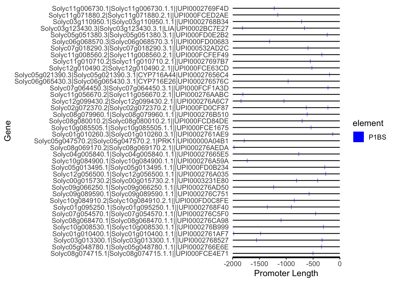
#p.P1BS + theme(line = element_line("blue")) # does not work
#p.P1BS + theme(plot.background = element_rect(color="blue")) # does not work

# how many genes ad P1BS?
SL.AMFcore.Zeng2023.P1BS.loc %>% count(ID) %>% dim() # 38 genes
## [1] 38 2length(SL.AMFcore.Zeng2023.gene) # 132 genes total## [1] 132# save
#ggsave(p.P1BS,file="promoter_motisf_P1BS_SL.AMFcore.Zeng2023.png",width=11,height=8)Session Info
sessionInfo()## R version 4.5.0 (2025-04-11)
## Platform: aarch64-apple-darwin20
## Running under: macOS Sonoma 14.8.2
##
## Matrix products: default
## BLAS: /Library/Frameworks/R.framework/Versions/4.5-arm64/Resources/lib/libRblas.0.dylib
## LAPACK: /Library/Frameworks/R.framework/Versions/4.5-arm64/Resources/lib/libRlapack.dylib; LAPACK version 3.12.1
##
## locale:
## [1] en_US.UTF-8/en_US.UTF-8/en_US.UTF-8/C/en_US.UTF-8/en_US.UTF-8
##
## time zone: America/Los_Angeles
## tzcode source: internal
##
## attached base packages:
## [1] stats graphics grDevices utils datasets methods base
##
## other attached packages:
## [1] BioVizSeq_1.0.4 lubridate_1.9.4 forcats_1.0.1
## [4] stringr_1.5.2 dplyr_1.1.4 purrr_1.1.0
## [7] readr_2.1.5 tidyr_1.3.1 tibble_3.3.0
## [10] ggplot2_4.0.0 tidyverse_2.0.0 shinydashboard_0.7.3
## [13] promises_1.5.0 htmltools_0.5.8.1
##
## loaded via a namespace (and not attached):
## [1] gtable_0.3.6 xfun_0.54 bslib_0.9.0 lattice_0.22-7
## [5] tzdb_0.5.0 vctrs_0.6.5 tools_4.5.0 generics_0.1.4
## [9] yulab.utils_0.2.1 parallel_4.5.0 pkgconfig_2.0.3 ggplotify_0.1.3
## [13] RColorBrewer_1.1-3 S7_0.2.0 readxl_1.4.5 lifecycle_1.0.4
## [17] compiler_4.5.0 farver_2.1.2 treeio_1.32.0 ggtree_3.16.3
## [21] httpuv_1.6.16 ggfun_0.2.0 sass_0.4.10 yaml_2.3.10
## [25] lazyeval_0.2.2 crayon_1.5.3 seqinr_4.2-36 later_1.4.4
## [29] pillar_1.11.1 jquerylib_0.1.4 MASS_7.3-65 cachem_1.1.0
## [33] mime_0.13 nlme_3.1-168 tidyselect_1.2.1 ggh4x_0.3.1
## [37] aplot_0.2.9 digest_0.6.37 stringi_1.8.7 bookdown_0.45
## [41] labeling_0.4.3 ade4_1.7-23 fastmap_1.2.0 grid_4.5.0
## [45] cli_3.6.5 magrittr_2.0.4 patchwork_1.3.2 ape_5.8-1
## [49] withr_3.0.2 scales_1.4.0 rappdirs_0.3.3 bit64_4.6.0-1
## [53] timechange_0.3.0 httr_1.4.7 rmarkdown_2.30 bit_4.6.0
## [57] otel_0.2.0 cellranger_1.1.0 blogdown_1.22 hms_1.1.4
## [61] shiny_1.11.1 evaluate_1.0.5 knitr_1.50 gridGraphics_0.5-1
## [65] rlang_1.1.6 Rcpp_1.1.0 xtable_1.8-4 glue_1.8.0
## [69] tidytree_0.4.6 vroom_1.6.6 rstudioapi_0.17.1 jsonlite_2.0.0
## [73] R6_2.6.1 fs_1.6.6