Download this Rmd file
Please download and modify your input/output file location
Download RNA-seq data from NCBI
Let’s use published RNA-seq data from Arabidopsis thaliana mutants (npr1-1 and npr4-4D) Ding (2018).
library(tidyverse)
library(stringr)
library(edgeR)
Trimming unnecessary sequences from data (such as adaptors) by trimmomatic
Needs to trim? Do fastqc and see results
trim?
# working in directories containing fastq files
fastfiles<-list.files(pattern="fastq")
system(paste("fastqc ",fastfiles,sep=""))
# and then check reports to see if there are adaptor contamination
# It seems those files were not contaminated so that no need to trim read files.
fastfiles.SE<- fastfiles %>% as_tibble() %>% separate(value,into=c("SRA","type","compress"),sep="\\.") %>% separate(SRA,into=c("SRA","pair"),sep="_") %>% group_by(SRA) %>%summarize(num=n()) %>% filter(num==1) %>% select(SRA) %>% as_vector()
# trim by trimmomatic (not necessary this time)
# system("makedir trimmed")
#for (x in fastfiles) {
#system(paste("trimmomatic.sh SE -threads 4 ",x," trimmed/trimmed_",x," ILLUMINACLIP:Bradseq_adapter.fa:2:30:10 LEADING:3 TRAILING:3 SLIDINGWINDOW:4:15 MINLEN:36",sep="")) # bug fixed
#}
# Or using inline loop?
#system("for i in *fastq.gz; do trimmomatic.sh SE -threads 4 $i trimmed/trimmed$i ILLUMINACLIP:Bradseq_adapter.fa:2:30:10 LEADING:3 TRAILING:3 SLIDINGWINDOW:4:15 MINLEN:36; done")
Mapping to reference cDNA and creating count data file (copied from Julin’s scripts “01_20170617_Map and normalize”)
read Kallisto manual https://pachterlab.github.io/kallisto/starting.html
Build index
#system("kallisto index -i TAIR10_cdna_20110103_representative_gene_model_kallisto_index TAIR10_cdna_20110103_representative_gene_model.gz")
# This reference seq has been updated in 2012! Redo mapping (101018)
#system("kallisto index -i TAIR10_cdna_20110103_representative_gene_model_updated_kallisto_index TAIR10_cdna_20110103_representative_gene_model_updated")
mapping
# makin directory for mapped
system("mkdir kallisto_sam_out2")
# reading fastq files
fastqfiles<-list.files(pattern="fastq.gz")
# fastq files with single end
fastqfiles.SE<- fastqfiles %>% as_tibble() %>% separate(value,into=c("SRA","type","compress"),sep="\\.") %>% separate(SRA,into=c("SRA","pair"),sep="_") %>% group_by(SRA) %>%summarize(num=n()) %>% filter(num==1) %>% select(SRA) %>% as_vector()
for(x in fastqfiles.SE) {
system(paste("kallisto quant -i TAIR10_cdna_20110103_representative_gene_model_updated_kallisto_index  -o kallisto_sam_out2/",x," --single -l 200 -s 40 --pseudobam ",x,"_1.fastq.gz | samtools view -Sb - > kallisto_sam_out2/",x,"/",x,".bam",sep=""))
setwd(paste("kallisto_sam_out2/",x,sep=""))
system(paste("samtools sort *.bam -o ",x,".sorted.bam",sep=""))
system("samtools index *.sorted.bam")
setwd("../../")
}
samtools view -u alignment.sam | samtools sort -@ 4 - output_prefix # https://www.biostars.org/p/263589/
Move the counts to my local computer # Julin used lftp (https://www.networkworld.com/article/2833203/operating-systems/unix--flexibly-moving-files-with-lftp.html)
#In my computer,
# lftp sftp://kazu@whitney.plb.ucdavis.edu
#  cd NGS/Ding_2018_Cell
#  mirror kallisto_sam_out2
remove unused files
system("cd  2018-10-01-differential-expression-analysis-with-public-available-sequencing-data_files/kallisto_sam_out2")
system("rm */*.json")
system("rm */*.bam*")
compress tsv files
system("gzip */abundance.tsv")Get counts into R
kallisto_files <- dir(path = "2018-10-01-differential-expression-analysis-with-public-available-sequencing-data_files/kallisto_sam_out2",pattern="abundance.tsv",recursive = TRUE,full.names = TRUE)
kallisto_files
getwd()
kallisto_files2<-list.files(path="2018-10-01-differential-expression-analysis-with-public-available-sequencing-data_files/kallisto_sam_out2")
kallisto_files2
kallisto_names <- str_split(kallisto_files,"/",simplify=TRUE)[,3]
kallisto_names
#combine count data in list
counts.list <- lapply(kallisto_files,read_tsv)
names(counts.list) <- kallisto_names
counts.list[[1]]
combine counts data
counts <- sapply(counts.list, dplyr::select, est_counts) %>%
  bind_cols(counts.list[[1]][,"target_id"],.)
counts[is.na(counts)] <- 0
colnames(counts) <- sub(".est_counts","",colnames(counts),fixed = TRUE)
counts
counts.updated<-counts

# write counts data
write_csv(counts.updated,"2018-10-01-differential-expression-analysis-with-public-available-sequencing-data_files/counts.updated.csv.gz")
sample info
#sample.info<-read_csv("2018-10-01-differential-expression-analysis-with-public-available-sequencing-data/SraRunInfo.csv")
sample.info<-read_csv("http://trace.ncbi.nlm.nih.gov/Traces/sra/sra.cgi?save=efetch&rettype=runinfo&db=sra&term=PRJNA434313") # Directly from ncbi site. This works!
## Parsed with column specification:
## cols(
## .default = col_character(),
## ReleaseDate = col_datetime(format = ""),
## LoadDate = col_datetime(format = ""),
## spots = col_integer(),
## bases = col_double(),
## spots_with_mates = col_integer(),
## avgLength = col_integer(),
## size_MB = col_integer(),
## InsertSize = col_integer(),
## InsertDev = col_integer(),
## Study_Pubmed_id = col_integer(),
## ProjectID = col_integer(),
## TaxID = col_integer()
## )## See spec(...) for full column specifications.sample.info2<-tibble(SampleName=c("GSM3014771","GSM3014772","GSM3014773","GSM3014774","GSM3014775","GSM3014776","GSM3014777","GSM3014778","GSM3014779","GSM3014780","GSM3014781","GSM3014782","GSM3014783","GSM3014784","GSM3014785","GSM3014786"),sample=c("WT_treated_1","WT_treated_2","WT_untreated_1","WT_untreated_2","npr1-1_treated_1","npr1-1_treated_2","npr1-1_untreated_1","npr1-1_untreated_2","npr4-4D_treated_1","npr4-4D_treated_2","npr4-4D_untreated_1","npr4-4D_untreated_2","npr1-1_npr4-4D_treated_1","npr1-1_npr4-4D_treated_2","npr1-1_npr4-4D_untreated_1","npr1-1_npr4-4D_untreated_2")) # # from https://www.ncbi.nlm.nih.gov/geo/query/acc.cgi?acc=GSE110702
# combine
sample.info.final <- left_join(sample.info,sample.info2,by="SampleName") %>% dplyr::select(Run,sample,LibraryLayout) %>% separate(sample,into=c("genotype1","genotype2","treatment","rep"),sep="_",fill="left",remove=FALSE) %>% unite(genotype,genotype1,genotype2,sep="_") %>% mutate(genotype=str_replace(genotype,"NA_","")) %>% unite(group,genotype,treatment,sep="_",remove=FALSE)check libraries by barplot and MDS plots
counts<-read_csv("2018-10-01-differential-expression-analysis-with-public-available-sequencing-data_files/counts.updated.csv.gz")## Parsed with column specification:
## cols(
## target_id = col_character(),
## SRR6739807 = col_double(),
## SRR6739808 = col_double(),
## SRR6739809 = col_double(),
## SRR6739810 = col_double(),
## SRR6739811 = col_double(),
## SRR6739812 = col_double(),
## SRR6739813 = col_double(),
## SRR6739814 = col_double(),
## SRR6739815 = col_double(),
## SRR6739816 = col_double(),
## SRR6739817 = col_double(),
## SRR6739818 = col_double()
## )all(colnames(counts)[-1]==sample.info.final[sample.info.final$LibraryLayout=="SINGLE","Run"])## [1] TRUEdge <- DGEList(counts[,-1],
group=as_vector(sample.info.final[sample.info.final$LibraryLayout=="SINGLE","group"]),
samples=sample.info.final[sample.info.final$LibraryLayout=="SINGLE",],
genes=counts$target_id)
# Filtering.
## From edgeR User guide (section 2.6. Filtering) "As a rule of thumb, genes are dropped if they can’t possibly be expressed in all the samples for any of the conditions. Users can set their own definition of genes being expressed. Usually a gene is required to have a count of 5-10 in a library to be considered expressed in that library. Users should also filter with count-per-million (CPM) rather than filtering on the counts directly, as the latter does not account for differences in library sizes between samples"
dge.nolow<-dge[rowSums(cpm(dge)> 5) >= 2,] # two replicates in this experiment.
table(rowSums(cpm(dge)> 5) >= 2) ##
## FALSE TRUE
## 16803 16799# normalization
dge.nolow <- calcNormFactors(dge.nolow)
# lib.size check
ggplot(dge.nolow$samples,aes(x=sample,y=norm.factors,fill=genotype)) + geom_col() +
theme(axis.text.x = element_text(angle=90, vjust=0.5,size = 7)) 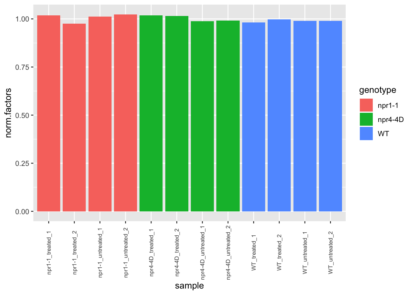
MDS plot
mds <- plotMDS(dge.nolow,method = "bcv",labels=dge.nolow$samples$group,gene.selection = "pairwise", ndim=3)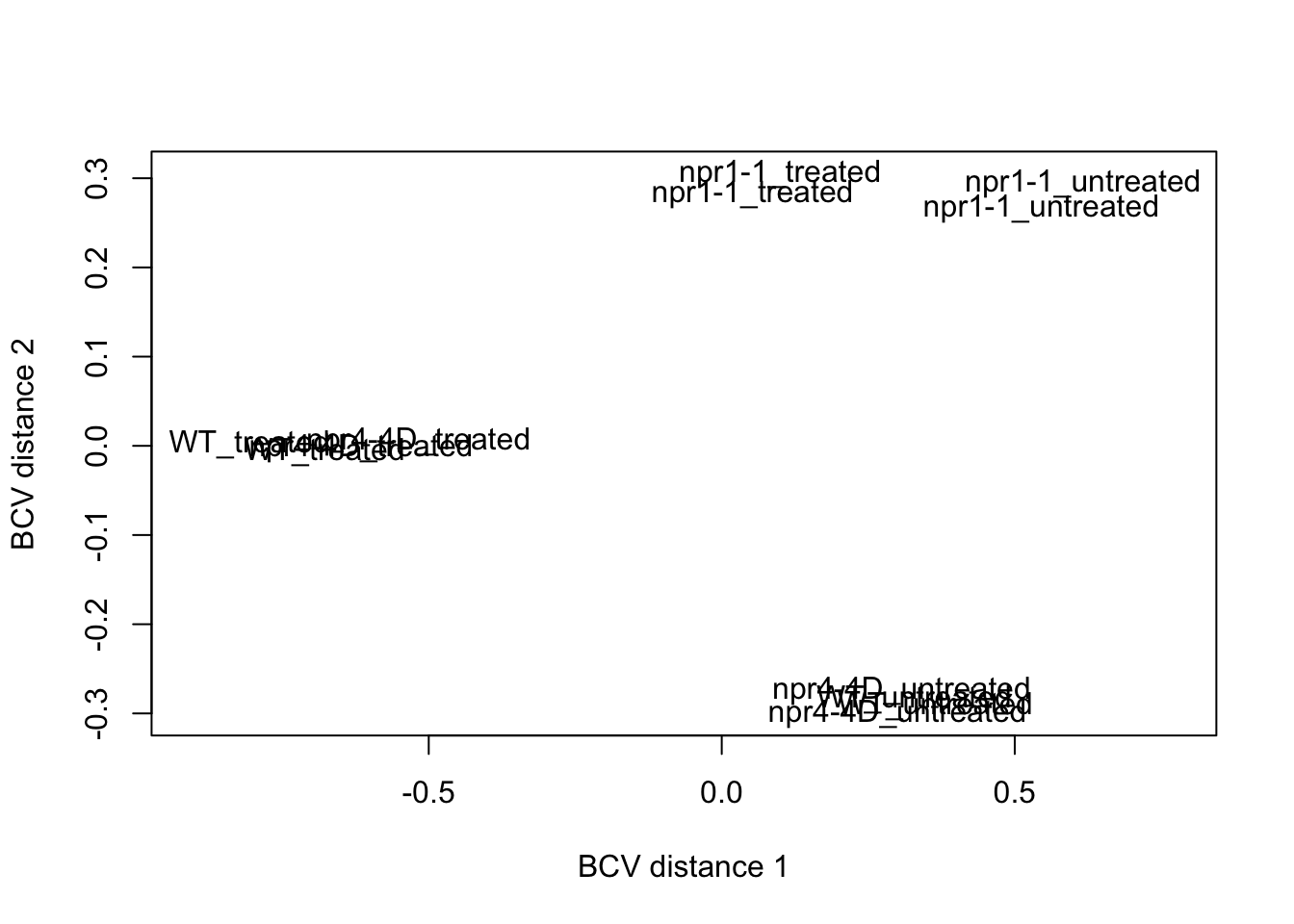
mds.pl <- as_tibble(mds$cmdscale.out) %>%
  bind_cols(data.frame(sample=row.names(mds$cmdscale.out)),.) %>%
  left_join(dge.nolow$sample,by=c(sample="Run"))
## Warning: Column `sample`/`Run` joining factor and character vector,
## coercing into character vectormds.pl %>% ggplot(aes(x=V1,y=V2,color=as.factor(treatment),label=genotype)) + geom_text(angle=30) + ggtitle("DIM 1 vs 2")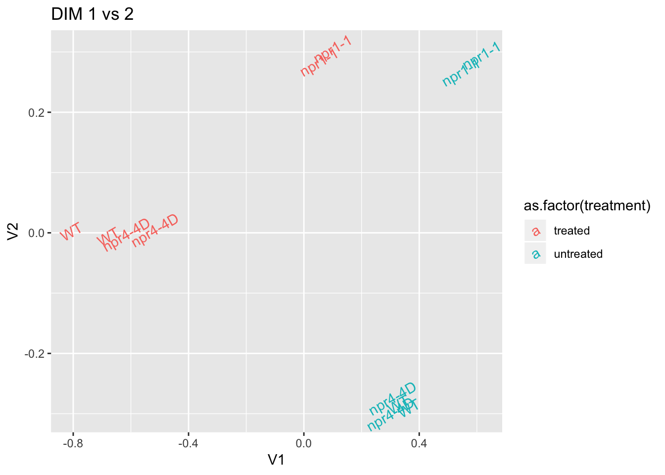 # edge.nolowR (model with glm)
# set references in genotype and treatment
dge.nolow$samples$genotype<-factor(dge.nolow$samples$genotype,levels=c("WT","npr4-4D","npr1-1"))
dge.nolow$samples$treatment<-factor(dge.nolow$samples$treatment,levels=c("untreated","treated"))
save(dge.nolow,file="2018-10-01-differential-expression-analysis-with-public-available-sequencing-data_files/dge.nolow.Ding2018.Rdata")
# making model matrix
design.int <- with(dge.nolow$samples, model.matrix(~ genotype*treatment + rep))
# estimateDisp
dge.nolow.int <- estimateDisp(dge.nolow,design = design.int)
## fit linear model
fit.int <- glmFit(dge.nolow.int,design.int)
# get DEGs, treatment effects in Col (rWT = reference WT, rU = reference is untreated)
trt.lrt.rWT.rU <- glmLRT(fit.int,coef = c("treatmenttreated"))
trt.DEGs.int.rWT.rU <- topTags(trt.lrt.rWT.rU,n = Inf,p.value = 0.05)$table;nrow(trt.DEGs.int.rWT.rU) #
## [1] 7862# get DEGs, genotype effects in npr1-1 (no matter treated or untreated) (coef=c("genotypenpr1-1","genotypenpr1-1:treatmenttreated"))
genotypenpr1_genotypenpr1.treatmenttreated.lrt.rWT.rU <- glmLRT(fit.int,coef = c("genotypenpr1-1","genotypenpr1-1:treatmenttreated"))
genotypenpr1_genotypenpr1.treatmenttreated.DEGs.int.rWT.rU <- topTags(genotypenpr1_genotypenpr1.treatmenttreated.lrt.rWT.rU,n = Inf,p.value = 0.05)$table;nrow(genotypenpr1_genotypenpr1.treatmenttreated.DEGs.int.rWT.rU) # ## [1] 6460# get DEGs, genotype effects in npr4-4D (no matter treated or untreated) (coef=c("genotypenpr4-4D","genotypenpr4-4D:treatmenttreated"))
genotypenpr4_genotypenpr4.treatmenttreated.lrt.rWT.rU <- glmLRT(fit.int,coef = c("genotypenpr4-4D","genotypenpr4-4D:treatmenttreated"))
genotypenpr4_genotypenpr4.treatmenttreated.DEGs.int.rWT.rU <- topTags(genotypenpr4_genotypenpr4.treatmenttreated.lrt.rWT.rU,n = Inf,p.value = 0.05)$table;nrow(genotypenpr4_genotypenpr4.treatmenttreated.DEGs.int.rWT.rU) # 846## [1] 854Download updated gene description
Most updated annotation can be downloaded from TAIR website (for subscribers). I used “TAIR Data 20180630”.
At.gene.name <-read_tsv("https://www.arabidopsis.org/download_files/Subscriber_Data_Releases/TAIR_Data_20180630/gene_aliases_20180702.txt.gz") # Does work from home when I use Pulse Secure.## Parsed with column specification:
## cols(
## name = col_character(),
## symbol = col_character(),
## full_name = col_character()
## )# test %>% dplyr::select(name,symbol) %>% group_by(name) %>% spread(key=name,value=symbol)
# test %>% dplyr::select(name,symbol) %>% spread(key=symbol,value=name)
# test %>% dplyr::select(name,symbol) %>% group_by(name) %>% spread(key=symbol,value=name)
# test %>% dplyr::select(name,symbol) %>% group_by(name) %>% summarise(n())
# How to concatenate multiple symbols in the same AGI
At.gene.name <- At.gene.name %>% group_by(name) %>% summarise(symbol2=paste(symbol,collapse=";"),full_name=paste(full_name,collapse=";"))
At.gene.name %>% dplyr::slice(100:110) # OK## # A tibble: 11 x 3
## name symbol2 full_name
## <chr> <chr> <chr>
## 1 AT1G018… AtGEN1;GEN1 NA;ortholog of HsGEN1
## 2 AT1G019… ATSBT1.1;SBTI1.1 NA;NA
## 3 AT1G019… AtGET3a;GET3a Guided Entry of Tail-anchored protein 3a;Gui…
## 4 AT1G019… ARK2;AtKINUb armadillo repeat kinesin 2;Arabidopsis thali…
## 5 AT1G019… BIG3;EDA10 BIG3;embryo sac development arrest 10
## 6 AT1G019… AtBBE1;OGOX4 NA;oligogalacturonide oxidase 4
## 7 AT1G020… GAE2 UDP-D-glucuronate 4-epimerase 2
## 8 AT1G020… SEC1A secretory 1A
## 9 AT1G020… LAP6;PKSA LESS ADHESIVE POLLEN 6;polyketide synthase A
## 10 AT1G020… SPL8 squamosa promoter binding protein-like 8
## 11 AT1G020… ATCSN7;COP15;CS… ARABIDOPSIS THALIANA COP9 SIGNALOSOME SUBUNI…Make “output” directory for saving DEG results as csv files
# system("mkdir 2018-10-01-differential-expression-analysis-with-public-available-sequencing-data_files/output")Add gene descripion to DEG files
# WT (Col) treatment DEG
trt.DEGs.int.rWT.rU.desc<- trt.DEGs.int.rWT.rU %>% mutate(AGI=str_remove(genes,pattern="\\.[[:digit:]]+$")) %>% left_join(At.gene.name,by=c("AGI"="name"))
write_csv(trt.DEGs.int.rWT.rU.desc,path="2018-10-01-differential-expression-analysis-with-public-available-sequencing-data_files/output/trt.DEGs.int.rWT.rU.csv")

# npr1-1 (either treated or untreated)
genotypenpr1_genotypenpr1.treatmenttreated.DEGs.int.rWT.rU.desc <- genotypenpr1_genotypenpr1.treatmenttreated.DEGs.int.rWT.rU %>% mutate(AGI=str_remove(genes,pattern="\\.[[:digit:]]+$")) %>% left_join(At.gene.name,by=c("AGI"="name"))
write_csv(genotypenpr1_genotypenpr1.treatmenttreated.DEGs.int.rWT.rU.desc,"2018-10-01-differential-expression-analysis-with-public-available-sequencing-data_files/output/genotypenpr1_genotypenpr1.treatmenttreated.DEGs.int.rWT.rU.csv")
# npr4-4 (either treated or untreated)
genotypenpr4_genotypenpr4.treatmenttreated.DEGs.int.rWT.rU.desc <- genotypenpr4_genotypenpr4.treatmenttreated.DEGs.int.rWT.rU %>% mutate(AGI=str_remove(genes,pattern="\\.[[:digit:]]+$")) %>% left_join(At.gene.name,by=c("AGI"="name"))
write_csv(genotypenpr4_genotypenpr4.treatmenttreated.DEGs.int.rWT.rU.desc,"2018-10-01-differential-expression-analysis-with-public-available-sequencing-data_files/output/genotypenpr4_genotypenpr4.treatmenttreated.DEGs.int.rWT.rU.csv")
table for DEGs summary
#DEG.objs<-list.files(path=file.path("2018-10-01-differential-expression-analysis-with-public-available-sequencing-data_files","output"),pattern="(DEGs)(.)(\\.csv)") # under construction
DEG.objs<-list.files(path=file.path("2018-10-01-differential-expression-analysis-with-public-available-sequencing-data_files","output"),pattern="\\.csv$") # under construction
DEG.objs
## [1] "genotypenpr1_genotypenpr1.treatmenttreated.DEGs.int.rWT.rU.csv"
## [2] "genotypenpr4_genotypenpr4.treatmenttreated.DEGs.int.rWT.rU.csv"
## [3] "trt.DEGs.int.rWT.rU.csv"# read csv file
DEG.count.list<-lapply(DEG.objs, function(x) read_csv(paste(file.path("2018-10-01-differential-expression-analysis-with-public-available-sequencing-data_files","output"),"/",x,sep="")))## Parsed with column specification:
## cols(
## genes = col_character(),
## logFC.genotypenpr1.1 = col_double(),
## logFC.genotypenpr1.1.treatmenttreated = col_double(),
## logCPM = col_double(),
## LR = col_double(),
## PValue = col_double(),
## FDR = col_double(),
## AGI = col_character(),
## symbol2 = col_character(),
## full_name = col_character()
## )## Parsed with column specification:
## cols(
## genes = col_character(),
## logFC.genotypenpr4.4D = col_double(),
## logFC.genotypenpr4.4D.treatmenttreated = col_double(),
## logCPM = col_double(),
## LR = col_double(),
## PValue = col_double(),
## FDR = col_double(),
## AGI = col_character(),
## symbol2 = col_character(),
## full_name = col_character()
## )## Parsed with column specification:
## cols(
## genes = col_character(),
## logFC = col_double(),
## logCPM = col_double(),
## LR = col_double(),
## PValue = col_double(),
## FDR = col_double(),
## AGI = col_character(),
## symbol2 = col_character(),
## full_name = col_character()
## )names(DEG.count.list)<-gsub(".csv","",DEG.objs)
DEGs.count<-sapply(DEG.count.list,function(x) {
value <- nrow(x)
ifelse(is.null(value),0,value)
} )
DEGs.count## genotypenpr1_genotypenpr1.treatmenttreated.DEGs.int.rWT.rU
## 6460
## genotypenpr4_genotypenpr4.treatmenttreated.DEGs.int.rWT.rU
## 854
## trt.DEGs.int.rWT.rU
## 7862Plot gene expression pattern
For some reasons, labeller = label_wrap_gen(width=30) does not work here. Needs to make a function for plotting graph later to reduce redundancy of scripts.
# calculate normalized gene expression level
cpm.wide <- bind_cols(dge.nolow$gene,as_tibble(cpm(dge.nolow))) %>% as_tibble() %>% rename(transcript_ID=genes)
cpm.wide
## # A tibble: 16,799 x 13
## transcript_ID SRR6739807 SRR6739808 SRR6739809 SRR6739810 SRR6739811
## <chr> <dbl> <dbl> <dbl> <dbl> <dbl>
## 1 AT1G50920.1 169. 164. 175. 158. 184.
## 2 AT1G15970.1 20.0 19.7 15.2 15.6 14.6
## 3 AT1G73440.1 6.22 6.17 7.39 6.33 7.10
## 4 AT1G75120.1 2.44 2.20 3.55 4.94 5.59
## 5 AT1G17600.1 32.1 36.5 11.1 9.87 12.1
## 6 AT1G77370.1 34.1 36.3 23.7 25.1 22.9
## 7 AT1G10950.1 172. 171. 133. 148. 173.
## 8 AT1G31870.1 40.8 38.5 26.8 26.9 33.3
## 9 AT1G51360.1 7.40 7.64 9.07 10.4 6.82
## 10 AT1G50950.1 4.45 4.49 3.74 5.16 5.50
## # ... with 16,789 more rows, and 7 more variables: SRR6739812 <dbl>,
## # SRR6739813 <dbl>, SRR6739814 <dbl>, SRR6739815 <dbl>,
## # SRR6739816 <dbl>, SRR6739817 <dbl>, SRR6739818 <dbl>#write_csv(cpm.wide,file.path("2018-10-01-differential-expression-analysis-with-public-available-sequencing-data_files","output","cpm_wide_Ding_2018_Cell.csv.gz"))
# plot
# format data for plot
plot.data<-DEG.count.list[["trt.DEGs.int.rWT.rU"]] %>% left_join(cpm.wide,by=c("genes"="transcript_ID")) %>% unite(AGI_desc,c("AGI","symbol2")) %>% dplyr::select(-LR,-PValue,-genes)
# plot: use labeller = label_wrap_gen(width=10) for multiple line in each gene name
p1<-plot.data %>% filter(logFC>0 & FDR<1e-100) %>% dplyr::select(-logFC,-logCPM,-FDR,-full_name) %>% gather(Run,value,-1) %>% left_join(sample.info.final,by="Run") %>% select(-Run,-sample,-group,-LibraryLayout) %>% ggplot(aes(x=fct_relevel(treatment,"untreated"),y=value,color=genotype,shape=rep)) + geom_jitter() + facet_wrap(AGI_desc~.,scale="free",ncol=5,labeller = label_wrap_gen(width=30))+theme(strip.text = element_text(size=6)) + labs(title="WT SA up-regulated genes")
p1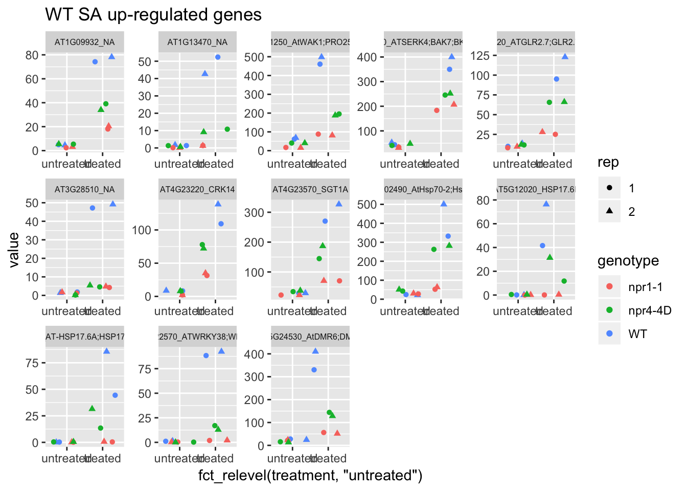
# SA down-regulated genes
plot.data2<-DEG.count.list[["trt.DEGs.int.rWT.rU"]] %>% left_join(cpm.wide,by=c("genes"="transcript_ID")) %>% unite(AGI_desc,c("AGI","symbol2")) %>% dplyr::select(-LR,-PValue,-genes)
# plot: use labeller = label_wrap_gen(width=10) for multiple line in each gene name
p2<-plot.data2 %>% filter(logFC<0 & FDR<1e-50) %>% dplyr::select(-logFC,-logCPM,-FDR,-full_name) %>% gather(Run,value,-1) %>% left_join(sample.info.final,by="Run") %>% select(-Run,-sample,-group,-LibraryLayout) %>% ggplot(aes(x=fct_relevel(treatment,"untreated"),y=value,color=genotype,shape=rep)) + geom_jitter() + facet_wrap(AGI_desc~.,scale="free",ncol=5,labeller = label_wrap_gen(width=30))+theme(strip.text = element_text(size=6)) + labs(title="WT SA down-regulated genes")
p2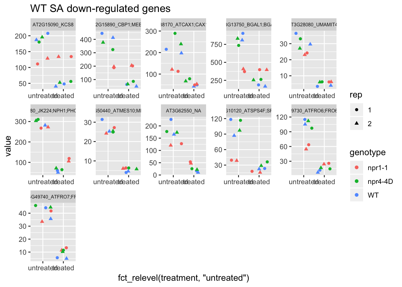 # npr1-1
# npr1-1 misregulated genes
plot.data3<-DEG.count.list[["genotypenpr1_genotypenpr1.treatmenttreated.DEGs.int.rWT.rU"]] %>% left_join(cpm.wide,by=c("genes"="transcript_ID")) %>% unite(AGI_desc,c("AGI","symbol2")) %>% dplyr::select(-LR,-PValue,-genes)
# plot: use labeller = label_wrap_gen(width=10) for multiple line in each gene name
p3<-plot.data3 %>% filter(logFC.genotypenpr1.1>0 & FDR<1e-100) %>% dplyr::select(-logFC.genotypenpr1.1,-logFC.genotypenpr1.1.treatmenttreated,-FDR,-full_name,-logCPM) %>%  gather(Run,value,-1) %>% left_join(sample.info.final,by="Run") %>% select(-Run,-sample,-group,-LibraryLayout) %>% ggplot(aes(x=fct_relevel(treatment,"untreated"),y=value,color=genotype,shape=rep)) + geom_jitter() + facet_wrap(AGI_desc~.,scale="free",ncol=5,labeller = label_wrap_gen(width=30))+theme(strip.text = element_text(size=6)) + labs(title="logFC.genotypenpr1.1>0")
p3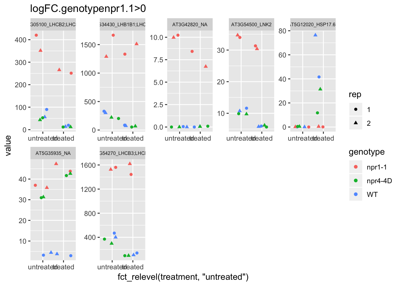
# plot: use labeller = label_wrap_gen(width=10) for multiple line in each gene name
p4<-plot.data3 %>% filter(logFC.genotypenpr1.1<0 & FDR<1e-100) %>% dplyr::select(-logFC.genotypenpr1.1,-logFC.genotypenpr1.1.treatmenttreated,-FDR,-full_name,-logCPM) %>%  gather(Run,value,-1) %>% left_join(sample.info.final,by="Run") %>% select(-Run,-sample,-group,-LibraryLayout) %>% ggplot(aes(x=fct_relevel(treatment,"untreated"),y=value,color=genotype,shape=rep)) + geom_jitter() + facet_wrap(AGI_desc~.,scale="free",ncol=5,labeller = label_wrap_gen(width=30))+theme(strip.text = element_text(size=6)) + labs(title="logFC.genotypenpr1.1<0")
p4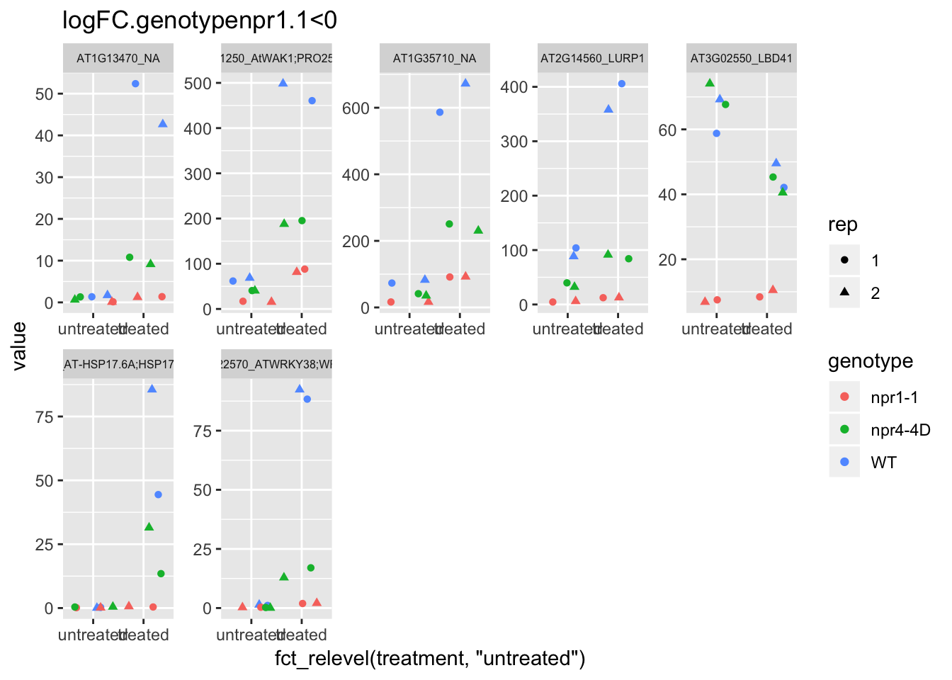
# plot: use labeller = label_wrap_gen(width=10) for multiple line in each gene name
p5<-plot.data3 %>% filter(logFC.genotypenpr1.1.treatmenttreated>0 & FDR<1e-100) %>% dplyr::select(-logFC.genotypenpr1.1,-logFC.genotypenpr1.1.treatmenttreated,-FDR,-full_name,-logCPM) %>%  gather(Run,value,-1) %>% left_join(sample.info.final,by="Run") %>% select(-Run,-sample,-group,-LibraryLayout) %>% ggplot(aes(x=fct_relevel(treatment,"untreated"),y=value,color=genotype,shape=rep)) + geom_jitter() + facet_wrap(AGI_desc~.,scale="free",ncol=5,labeller = label_wrap_gen(width=30))+theme(strip.text = element_text(size=6)) + labs(title="logFC.genotypenpr1.1.treatmenttreated>0")
p5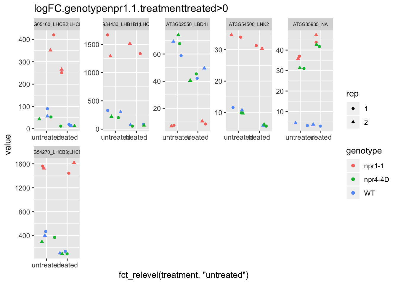
# plot: use labeller = label_wrap_gen(width=10) for multiple line in each gene name
p6<-plot.data3 %>% filter(logFC.genotypenpr1.1.treatmenttreated<0 & FDR<1e-100) %>% dplyr::select(-logFC.genotypenpr1.1,-logFC.genotypenpr1.1.treatmenttreated,-FDR,-full_name,-logCPM) %>%  gather(Run,value,-1) %>% left_join(sample.info.final,by="Run") %>% select(-Run,-sample,-group,-LibraryLayout) %>% ggplot(aes(x=fct_relevel(treatment,"untreated"),y=value,color=genotype,shape=rep)) + geom_jitter() + facet_wrap(AGI_desc~.,scale="free",ncol=5,labeller = label_wrap_gen(width=30))+theme(strip.text = element_text(size=6)) + labs(title="logFC.genotypenpr1.1.treatmenttreated<0")
p6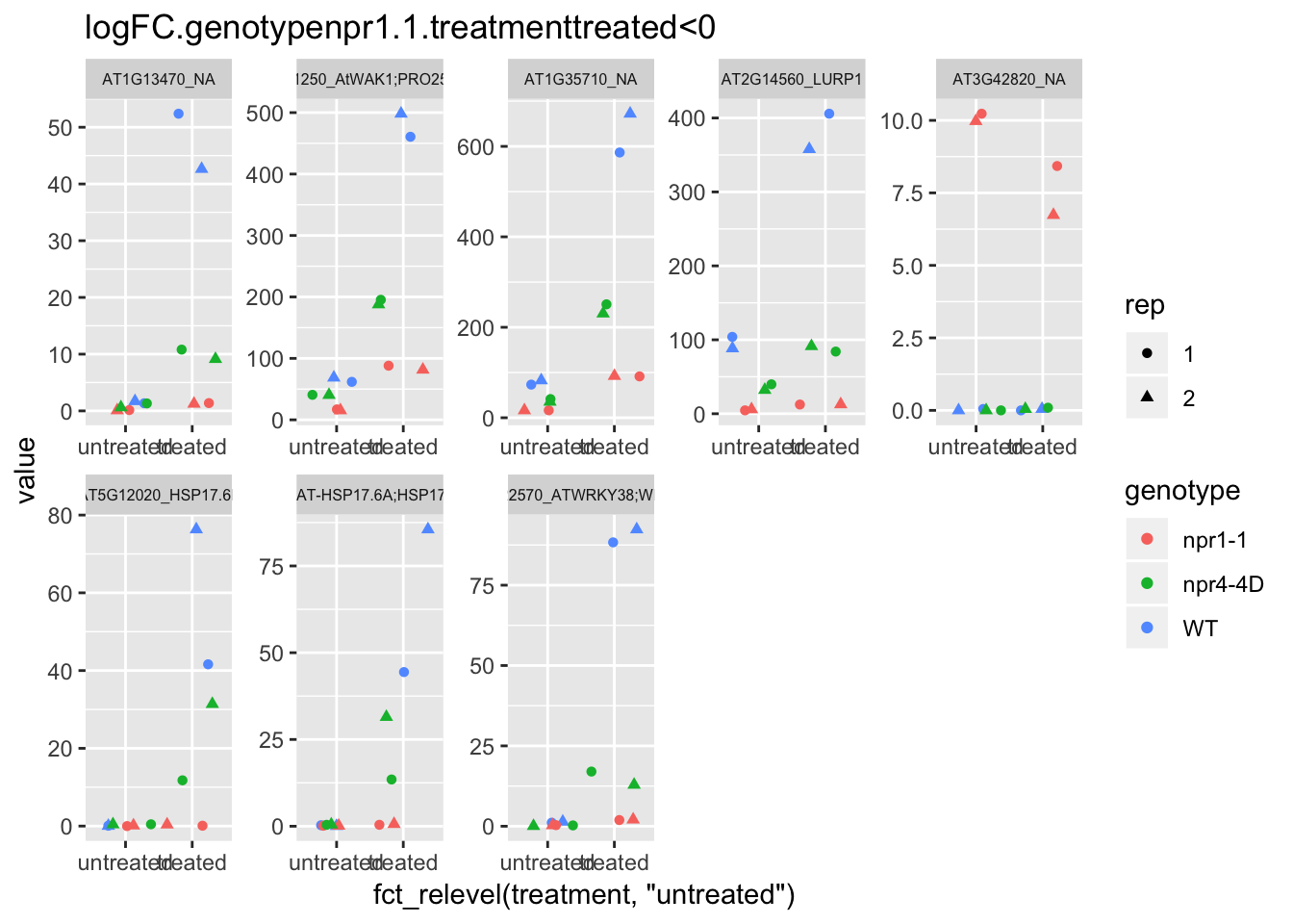
Session info
sessionInfo()## R version 3.5.1 (2018-07-02)
## Platform: x86_64-apple-darwin15.6.0 (64-bit)
## Running under: macOS 10.14.1
##
## Matrix products: default
## BLAS: /Library/Frameworks/R.framework/Versions/3.5/Resources/lib/libRblas.0.dylib
## LAPACK: /Library/Frameworks/R.framework/Versions/3.5/Resources/lib/libRlapack.dylib
##
## locale:
## [1] en_US.UTF-8/en_US.UTF-8/en_US.UTF-8/C/en_US.UTF-8/en_US.UTF-8
##
## attached base packages:
## [1] stats graphics grDevices utils datasets methods base
##
## other attached packages:
## [1] bindrcpp_0.2.2 edgeR_3.22.5 limma_3.36.5 forcats_0.3.0
## [5] stringr_1.3.1 dplyr_0.7.7 purrr_0.2.5 readr_1.1.1
## [9] tidyr_0.8.2 tibble_1.4.2 ggplot2_3.1.0 tidyverse_1.2.1
##
## loaded via a namespace (and not attached):
## [1] tidyselect_0.2.5 locfit_1.5-9.1 xfun_0.4 splines_3.5.1
## [5] haven_1.1.2 lattice_0.20-35 colorspace_1.3-2 htmltools_0.3.6
## [9] yaml_2.2.0 utf8_1.1.4 rlang_0.3.0.1 pillar_1.3.0
## [13] glue_1.3.0 withr_2.1.2 modelr_0.1.2 readxl_1.1.0
## [17] bindr_0.1.1 plyr_1.8.4 munsell_0.5.0 blogdown_0.10
## [21] gtable_0.2.0 cellranger_1.1.0 rvest_0.3.2 evaluate_0.12
## [25] labeling_0.3 knitr_1.21 curl_3.2 fansi_0.4.0
## [29] broom_0.5.0 Rcpp_1.0.0 scales_1.0.0 backports_1.1.2
## [33] jsonlite_1.6 hms_0.4.2 digest_0.6.18 stringi_1.2.4
## [37] bookdown_0.9 grid_3.5.1 cli_1.0.1 tools_3.5.1
## [41] magrittr_1.5 lazyeval_0.2.1 crayon_1.3.4 pkgconfig_2.0.2
## [45] xml2_1.2.0 lubridate_1.7.4 assertthat_0.2.0 rmarkdown_1.11
## [49] httr_1.3.1 rstudioapi_0.8 R6_2.3.0 nlme_3.1-137
## [53] compiler_3.5.1