Hierarchical clustering is powerful method to classify gene expression pattern. Here I applied a method develped by an example of plotly.
Required libraries
# install.packages('ggdendro')
library(tidyverse);library(ggdendro);library(plotly)
Reading expression value
# reading gene expression value (Ding, 2018) from my privious blog (["Differential expression analysis with public available sequencing data"](https://knozue.github.io/post/2018/10/01/differential-expression-analysis-with-public-available-sequencing-data.html) on 2018-10-01))
load(file.path("..","..","..","resources","2018-10-24-dge-clustering-with-ggplot2_files","dge.nolow.Ding2018.Rdata"))
dge.nolow
## Loading required package: edgeR## Loading required package: limma## An object of class "DGEList"
## $counts
## SRR6739807 SRR6739808 SRR6739809 SRR6739810 SRR6739811 SRR6739812 SRR6739813
## 1 3598.000 3442.000 3653 3531 4027 3775 4195
## 4 427.000 412.000 316 348 319 357 286
## 5 132.805 129.168 154 141 155 131 126
## 6 52.000 46.000 74 110 122 91 118
## 7 685.000 764.000 231 220 264 247 118
## SRR6739814 SRR6739815 SRR6739816 SRR6739817 SRR6739818
## 1 4317.9900 4015.000 3874.000 3663.000 3642
## 4 306.0000 389.000 362.000 290.000 285
## 5 99.8598 156.895 130.783 101.738 120
## 6 135.0000 60.000 52.000 85.000 79
## 7 131.0000 416.000 383.000 104.000 164
## 16794 more rows ...
##
## $samples
## group lib.size norm.factors Run sample
## SRR6739807 WT_treated 21747803 0.9813040 SRR6739807 WT_treated_1
## SRR6739808 WT_treated 21005249 0.9969243 SRR6739808 WT_treated_2
## SRR6739809 WT_untreated 21052743 0.9901012 SRR6739809 WT_untreated_1
## SRR6739810 WT_untreated 22518666 0.9893923 SRR6739810 WT_untreated_2
## SRR6739811 npr1-1_treated 21437014 1.0185940 SRR6739811 npr1-1_treated_1
## group.1 genotype treatment rep LibraryLayout
## SRR6739807 WT_treated WT treated 1 SINGLE
## SRR6739808 WT_treated WT treated 2 SINGLE
## SRR6739809 WT_untreated WT untreated 1 SINGLE
## SRR6739810 WT_untreated WT untreated 2 SINGLE
## SRR6739811 npr1-1_treated npr1-1 treated 1 SINGLE
## 7 more rows ...
##
## $genes
## genes
## 1 AT1G50920.1
## 4 AT1G15970.1
## 5 AT1G73440.1
## 6 AT1G75120.1
## 7 AT1G17600.1
## 16794 more rows ...cpm.wide <- bind_cols(dge.nolow$gene,as_tibble(cpm(dge.nolow))) %>% as_tibble() %>% rename(transcript_ID=genes)
cpm.wide## # A tibble: 16,799 x 13
## transcript_ID SRR6739807 SRR6739808 SRR6739809 SRR6739810 SRR6739811
## <chr> <dbl> <dbl> <dbl> <dbl> <dbl>
## 1 AT1G50920.1 169. 164. 175. 158. 184.
## 2 AT1G15970.1 20.0 19.7 15.2 15.6 14.6
## 3 AT1G73440.1 6.22 6.17 7.39 6.33 7.10
## 4 AT1G75120.1 2.44 2.20 3.55 4.94 5.59
## 5 AT1G17600.1 32.1 36.5 11.1 9.87 12.1
## 6 AT1G77370.1 34.1 36.3 23.7 25.1 22.9
## 7 AT1G10950.1 172. 171. 133. 148. 173.
## 8 AT1G31870.1 40.8 38.5 26.8 26.9 33.3
## 9 AT1G51360.1 7.40 7.64 9.07 10.4 6.82
## 10 AT1G50950.1 4.45 4.49 3.74 5.16 5.50
## # … with 16,789 more rows, and 7 more variables: SRR6739812 <dbl>,
## # SRR6739813 <dbl>, SRR6739814 <dbl>, SRR6739815 <dbl>, SRR6739816 <dbl>,
## # SRR6739817 <dbl>, SRR6739818 <dbl>DGE list of interest
This example uses misexpressed genes in salicilyc acid treatment and/or in salicylic acid related mutants (npe1-1 and npr4-D) reported in Ding (2018), which RNAseq data are reanlized in my blog.
# Ding (2018) Cell DEGs
DEG.objs<-list.files(path=file.path("..","..","..","resources","2018-10-24-dge-clustering-with-ggplot2_files","output_copy_DEG"),pattern="\\.csv$",full.names=TRUE,recursive=TRUE) # under construction
DEG.objs
## [1] "../../../resources/2018-10-24-dge-clustering-with-ggplot2_files/output_copy_DEG/genotypenpr1_genotypenpr1.treatmenttreated.DEGs.int.rWT.rU.csv"
## [2] "../../../resources/2018-10-24-dge-clustering-with-ggplot2_files/output_copy_DEG/genotypenpr4_genotypenpr4.treatmenttreated.DEGs.int.rWT.rU.csv"
## [3] "../../../resources/2018-10-24-dge-clustering-with-ggplot2_files/output_copy_DEG/trt.DEGs.int.rWT.rU.csv"# read csv file
DEG.list <- DEG.objs %>% map(~read_csv(.))##
## ── Column specification ────────────────────────────────────────────────────────
## cols(
## genes = col_character(),
## logFC.genotypenpr1.1 = col_double(),
## logFC.genotypenpr1.1.treatmenttreated = col_double(),
## logCPM = col_double(),
## LR = col_double(),
## PValue = col_double(),
## FDR = col_double(),
## AGI = col_character(),
## symbol2 = col_character(),
## full_name = col_character()
## )##
## ── Column specification ────────────────────────────────────────────────────────
## cols(
## genes = col_character(),
## logFC.genotypenpr4.4D = col_double(),
## logFC.genotypenpr4.4D.treatmenttreated = col_double(),
## logCPM = col_double(),
## LR = col_double(),
## PValue = col_double(),
## FDR = col_double(),
## AGI = col_character(),
## symbol2 = col_character(),
## full_name = col_character()
## )##
## ── Column specification ────────────────────────────────────────────────────────
## cols(
## genes = col_character(),
## logFC = col_double(),
## logCPM = col_double(),
## LR = col_double(),
## PValue = col_double(),
## FDR = col_double(),
## AGI = col_character(),
## symbol2 = col_character(),
## full_name = col_character()
## )names(DEG.list) <- str_split(DEG.objs,pattern="/",simplify=TRUE)[,7] %>% str_remove(".csv")
head(DEG.list)## $genotypenpr1_genotypenpr1.treatmenttreated.DEGs.int.rWT.rU
## # A tibble: 6,460 x 10
## genes logFC.genotypen… logFC.genotypen… logCPM LR PValue FDR
## <chr> <dbl> <dbl> <dbl> <dbl> <dbl> <dbl>
## 1 AT2G… -4.19 -0.733 6.69 1327. 6.75e-289 1.13e-284
## 2 AT5G… 3.26 0.517 4.76 1072. 1.33e-233 1.11e-229
## 3 AT1G… -2.01 -0.488 7.19 659. 6.38e-144 3.57e-140
## 4 AT1G… -2.25 -0.525 7.51 624. 2.54e-136 1.07e-132
## 5 AT3G… -3.15 0.874 5.33 622. 1.00e-135 3.36e-132
## 6 AT5G… -0.206 -6.73 3.90 595. 7.88e-130 2.21e-126
## 7 AT1G… -3.64 -1.53 3.37 581. 7.28e-127 1.75e-123
## 8 AT5G… 1.83 1.82 9.40 571. 1.04e-124 2.18e-121
## 9 AT2G… 2.23 1.94 9.22 559. 4.26e-122 7.94e-119
## 10 AT5G… -2.01 -3.49 4.19 538. 1.19e-117 2.00e-114
## # … with 6,450 more rows, and 3 more variables: AGI <chr>, symbol2 <chr>,
## # full_name <chr>
##
## $genotypenpr4_genotypenpr4.treatmenttreated.DEGs.int.rWT.rU
## # A tibble: 854 x 10
## genes logFC.genotypen… logFC.genotypen… logCPM LR PValue FDR
## <chr> <dbl> <dbl> <dbl> <dbl> <dbl> <dbl>
## 1 AT5G… 3.04 0.632 4.76 966. 1.54e-210 2.59e-206
## 2 AT5G… -3.31 0.358 3.10 463. 3.40e-101 2.85e- 97
## 3 AT3G… -5.46 -0.178 1.98 454. 2.07e- 99 1.16e- 95
## 4 AT1G… -7.41 -3.70 2.00 424. 6.68e- 93 2.80e- 89
## 5 AT3G… -2.97 -0.297 3.36 393. 4.39e- 86 1.47e- 82
## 6 AT2G… -1.42 -0.699 6.69 284. 2.63e- 62 7.35e- 59
## 7 AT1G… -2.50 0.894 6.30 280. 1.23e- 61 2.96e- 58
## 8 AT2G… -1.10 -0.233 5.87 221. 9.62e- 49 2.02e- 45
## 9 AT5G… -3.04 0.438 4.19 208. 6.15e- 46 1.15e- 42
## 10 AT5G… -1.84 -0.485 2.78 190. 4.64e- 42 7.79e- 39
## # … with 844 more rows, and 3 more variables: AGI <chr>, symbol2 <chr>,
## # full_name <chr>
##
## $trt.DEGs.int.rWT.rU
## # A tibble: 7,862 x 9
## genes logFC logCPM LR PValue FDR AGI symbol2 full_name
## <chr> <dbl> <dbl> <dbl> <dbl> <dbl> <chr> <chr> <chr>
## 1 AT5G1… 8.58 3.90 662. 5.49e-146 9.22e-142 AT5G1… AT-HSP1… heat shock pro…
## 2 AT1G0… 4.01 4.60 613. 2.14e-135 1.80e-131 AT1G0… <NA> <NA>
## 3 AT4G2… 3.86 5.39 586. 2.36e-129 1.32e-125 AT4G2… CRK14 cysteine-rich …
## 4 AT5G2… 6.17 4.19 582. 1.27e-128 5.32e-125 AT5G2… ATWRKY3… ARABIDOPSIS TH…
## 5 AT3G2… 4.93 3.36 578. 9.46e-128 3.18e-124 AT3G2… <NA> <NA>
## 6 AT5G1… 9.65 3.77 569. 1.18e-125 3.30e-122 AT5G1… HSP17.6… 17.6 kDa class…
## 7 AT4G2… 3.34 6.70 563. 1.80e-124 4.32e-121 AT4G2… SGT1A <NA>
## 8 AT1G2… 2.88 7.19 539. 2.54e-119 5.34e-116 AT1G2… AtWAK1;… NA;NA;cell wal…
## 9 AT5G2… 3.83 6.70 529. 4.88e-117 9.12e-114 AT5G2… AtDMR6;… NA;DOWNY MILDE…
## 10 AT2G1… 2.96 7.30 512. 2.22e-113 3.73e-110 AT2G1… ATSERK4… SOMATIC EMBRYO…
## # … with 7,852 more rowsmaking matrix for DEGs
DEG.genes<-unique(as_vector(rbind(DEG.list[[1]][DEG.list[[1]]$FDR<1e-30,"genes"],
                                DEG.list[[2]][DEG.list[[2]]$FDR<1e-30,"genes"],
                                DEG.list[[3]][DEG.list[[3]]$FDR<1e-30,"genes"])))
DEG.DF<- cpm.wide %>% filter(transcript_ID %in% DEG.genes)
dim(DEG.DF) # 305 13
## [1] 305 13sample info
#sample.info<-read_csv("2018-10-01-differential-expression-analysis-with-public-available-sequencing-data/SraRunInfo.csv")
sample.info<-read_csv("http://trace.ncbi.nlm.nih.gov/Traces/sra/sra.cgi?save=efetch&rettype=runinfo&db=sra&term=PRJNA434313") # Directly from ncbi site. This works!
##
## ── Column specification ────────────────────────────────────────────────────────
## cols(
## .default = col_character(),
## ReleaseDate = col_datetime(format = ""),
## LoadDate = col_datetime(format = ""),
## spots = col_double(),
## bases = col_double(),
## spots_with_mates = col_double(),
## avgLength = col_double(),
## size_MB = col_double(),
## AssemblyName = col_logical(),
## LibraryName = col_logical(),
## InsertSize = col_double(),
## InsertDev = col_double(),
## Study_Pubmed_id = col_double(),
## ProjectID = col_double(),
## TaxID = col_double(),
## g1k_pop_code = col_logical(),
## source = col_logical(),
## g1k_analysis_group = col_logical(),
## Subject_ID = col_logical(),
## Sex = col_logical(),
## Disease = col_logical()
## # ... with 5 more columns
## )
## ℹ Use `spec()` for the full column specifications.sample.info2<-tibble(SampleName=c("GSM3014771","GSM3014772","GSM3014773","GSM3014774","GSM3014775","GSM3014776","GSM3014777","GSM3014778","GSM3014779","GSM3014780","GSM3014781","GSM3014782","GSM3014783","GSM3014784","GSM3014785","GSM3014786"),sample=c("WT_treated_1","WT_treated_2","WT_untreated_1","WT_untreated_2","npr1-1_treated_1","npr1-1_treated_2","npr1-1_untreated_1","npr1-1_untreated_2","npr4-4D_treated_1","npr4-4D_treated_2","npr4-4D_untreated_1","npr4-4D_untreated_2","npr1-1_npr4-4D_treated_1","npr1-1_npr4-4D_treated_2","npr1-1_npr4-4D_untreated_1","npr1-1_npr4-4D_untreated_2")) # # from https://www.ncbi.nlm.nih.gov/geo/query/acc.cgi?acc=GSE110702
# combine
sample.info.final <- left_join(sample.info,sample.info2,by="SampleName") %>% dplyr::select(Run,sample,LibraryLayout) %>% separate(sample,into=c("genotype1","genotype2","treatment","rep"),sep="_",fill="left",remove=FALSE) %>% unite(genotype,genotype1,genotype2,sep="_") %>% mutate(genotype=str_replace(genotype,"NA_","")) %>% unite(group,genotype,treatment,sep="_",remove=FALSE)An example (under construction; there is a bug)
#dendogram data
x <- as.matrix(scale(t(DEG.DF[,-1]), center=T, scale=F))
dd.col.gene <- as.dendrogram(hclust(dist(x)))
dd.row.sample <- as.dendrogram(hclust(dist(t(x))))
dx <- dendro_data(dd.row.sample)
dy <- dendro_data(dd.col.gene)

# helper function for creating dendograms
ggdend <- function(df) {
  ggplot() +
    geom_segment(data = df, aes(x=x, y=y, xend=xend, yend=yend)) +
    labs(x = "", y = "") + theme_minimal() +
    theme(axis.text = element_blank(), axis.ticks = element_blank(),
          panel.grid = element_blank())
}

# x/y dendograms
px <- ggdend(dx$segments)
py <- ggdend(dy$segments) + coord_flip()
heatmap
col.ord <- order.dendrogram(dd.col.gene)
row.ord <- order.dendrogram(dd.row.sample)
df <- as.data.frame(x)
rowSums(df);colSums(df)
## SRR6739807 SRR6739808 SRR6739809 SRR6739810 SRR6739811 SRR6739812
## 12653.2472 17435.3104 -7424.3251 -9163.1272 2365.7416 5615.4999
## SRR6739813 SRR6739814 SRR6739815 SRR6739816 SRR6739817 SRR6739818
## -522.9579 -2443.7306 -536.5553 2588.6571 -10302.6584 -10265.1015## V1 V2 V3 V4 V5
## -3.907985e-14 3.108624e-15 -1.998401e-15 4.263256e-14 -1.154632e-14
## V6 V7 V8 V9 V10
## 1.065814e-14 6.394885e-14 -2.842171e-14 1.421085e-14 3.197442e-14
## V11 V12 V13 V14 V15
## -7.105427e-15 8.881784e-15 1.421085e-14 9.947598e-14 -9.094947e-13
## V16 V17 V18 V19 V20
## -7.105427e-15 2.842171e-14 -3.552714e-14 -3.126388e-13 8.881784e-16
## V21 V22 V23 V24 V25
## -1.421085e-14 1.421085e-14 -1.776357e-14 0.000000e+00 2.273737e-13
## V26 V27 V28 V29 V30
## -1.136868e-13 -7.815970e-14 1.136868e-13 3.552714e-14 1.136868e-13
## V31 V32 V33 V34 V35
## -1.136868e-13 -1.421085e-13 3.552714e-14 3.552714e-14 0.000000e+00
## V36 V37 V38 V39 V40
## 1.243450e-14 5.684342e-14 2.131628e-14 -4.263256e-14 1.776357e-14
## V41 V42 V43 V44 V45
## 4.440892e-15 -1.421085e-14 -1.705303e-13 1.421085e-14 -1.776357e-15
## V46 V47 V48 V49 V50
## -7.105427e-15 0.000000e+00 6.217249e-15 -2.309264e-14 -1.065814e-14
## V51 V52 V53 V54 V55
## 1.953993e-14 1.776357e-15 3.552714e-14 8.526513e-14 -1.776357e-14
## V56 V57 V58 V59 V60
## -1.598721e-14 1.421085e-14 -1.563194e-13 -7.105427e-14 1.136868e-13
## V61 V62 V63 V64 V65
## -2.842171e-14 1.243450e-14 8.526513e-14 1.563194e-13 -4.263256e-14
## V66 V67 V68 V69 V70
## 5.684342e-14 2.842171e-14 -7.105427e-15 -9.947598e-14 -1.136868e-13
## V71 V72 V73 V74 V75
## -3.907985e-14 5.329071e-15 1.598721e-14 2.842171e-14 -8.881784e-16
## V76 V77 V78 V79 V80
## 1.136868e-13 -8.526513e-14 -5.329071e-15 -3.552714e-15 -7.105427e-15
## V81 V82 V83 V84 V85
## -1.136868e-13 -5.684342e-14 3.552714e-15 1.065814e-14 -1.421085e-14
## V86 V87 V88 V89 V90
## -4.618528e-14 -4.973799e-14 7.105427e-15 5.329071e-15 6.252776e-13
## V91 V92 V93 V94 V95
## -8.526513e-14 -3.979039e-13 5.329071e-15 2.131628e-14 -7.105427e-15
## V96 V97 V98 V99 V100
## 3.197442e-14 -2.842171e-14 2.131628e-14 7.815970e-14 -3.552714e-15
## V101 V102 V103 V104 V105
## -1.065814e-14 0.000000e+00 1.421085e-14 5.329071e-15 -1.023182e-12
## V106 V107 V108 V109 V110
## -7.105427e-14 3.552714e-15 5.329071e-15 4.263256e-14 -3.197442e-14
## V111 V112 V113 V114 V115
## -7.105427e-14 -4.440892e-15 -1.332268e-15 4.440892e-15 -1.421085e-14
## V116 V117 V118 V119 V120
## 2.842171e-14 -1.776357e-15 -5.684342e-14 8.881784e-15 1.776357e-14
## V121 V122 V123 V124 V125
## 7.105427e-14 -4.263256e-14 -2.557954e-13 -2.273737e-13 1.243450e-14
## V126 V127 V128 V129 V130
## 2.486900e-14 4.263256e-14 7.105427e-14 -1.421085e-14 3.552714e-15
## V131 V132 V133 V134 V135
## -1.065814e-14 1.065814e-14 -7.105427e-15 -2.442491e-15 -4.440892e-16
## V136 V137 V138 V139 V140
## -1.136868e-13 -1.776357e-15 3.552714e-15 -9.769963e-15 0.000000e+00
## V141 V142 V143 V144 V145
## 3.979039e-13 -6.394885e-14 -4.440892e-16 -4.263256e-14 -2.273737e-13
## V146 V147 V148 V149 V150
## 4.440892e-15 2.842171e-14 -6.217249e-15 1.065814e-14 6.394885e-14
## V151 V152 V153 V154 V155
## -5.684342e-14 -2.131628e-14 1.065814e-14 1.023182e-12 -5.329071e-15
## V156 V157 V158 V159 V160
## -2.131628e-14 -1.776357e-15 5.329071e-15 3.552714e-15 2.842171e-14
## V161 V162 V163 V164 V165
## 4.440892e-16 -1.421085e-14 -7.105427e-15 -8.881784e-15 -7.105427e-15
## V166 V167 V168 V169 V170
## 2.842171e-14 -4.440892e-16 -1.421085e-14 -2.842171e-14 3.552714e-14
## V171 V172 V173 V174 V175
## 0.000000e+00 7.105427e-14 7.105427e-14 8.881784e-15 1.421085e-14
## V176 V177 V178 V179 V180
## -1.421085e-13 1.250555e-12 -1.598721e-14 -1.598721e-14 0.000000e+00
## V181 V182 V183 V184 V185
## -1.243450e-14 2.664535e-15 -1.421085e-14 1.421085e-14 8.881784e-16
## V186 V187 V188 V189 V190
## -1.421085e-14 -7.105427e-15 1.421085e-14 -4.263256e-14 1.421085e-14
## V191 V192 V193 V194 V195
## 2.664535e-15 -1.563194e-13 -7.105427e-15 -1.421085e-14 -1.065814e-14
## V196 V197 V198 V199 V200
## 3.126388e-13 -1.278977e-13 2.131628e-14 -7.105427e-15 1.421085e-13
## V201 V202 V203 V204 V205
## -2.664535e-15 2.842171e-14 1.776357e-15 -8.881784e-15 2.842171e-14
## V206 V207 V208 V209 V210
## -3.552714e-15 2.842171e-14 -2.664535e-15 2.842171e-14 -2.842171e-14
## V211 V212 V213 V214 V215
## 1.421085e-14 -1.421085e-14 -5.329071e-15 1.065814e-14 1.421085e-14
## V216 V217 V218 V219 V220
## -1.421085e-13 0.000000e+00 -5.329071e-15 -2.273737e-13 8.881784e-15
## V221 V222 V223 V224 V225
## -1.421085e-14 0.000000e+00 -1.776357e-14 5.329071e-15 2.486900e-14
## V226 V227 V228 V229 V230
## 2.842171e-14 -1.421085e-14 -1.421085e-14 2.842171e-14 7.815970e-14
## V231 V232 V233 V234 V235
## -1.776357e-14 -1.776357e-15 -1.421085e-14 -1.421085e-14 -3.552714e-15
## V236 V237 V238 V239 V240
## -8.881784e-15 2.842171e-14 -3.552714e-14 8.881784e-15 -2.486900e-14
## V241 V242 V243 V244 V245
## 2.664535e-15 -3.907985e-14 -3.410605e-13 3.552714e-15 -8.881784e-16
## V246 V247 V248 V249 V250
## 1.776357e-14 0.000000e+00 -1.421085e-14 1.421085e-14 -5.329071e-15
## V251 V252 V253 V254 V255
## 2.273737e-13 8.881784e-16 -2.131628e-14 1.136868e-13 -1.776357e-15
## V256 V257 V258 V259 V260
## -2.842171e-14 8.526513e-14 -1.776357e-15 -4.263256e-14 7.105427e-14
## V261 V262 V263 V264 V265
## -1.065814e-14 8.881784e-16 3.197442e-14 -1.421085e-14 5.684342e-14
## V266 V267 V268 V269 V270
## 1.421085e-14 1.421085e-14 -1.421085e-14 -7.105427e-14 7.105427e-14
## V271 V272 V273 V274 V275
## -1.776357e-14 -8.526513e-14 -3.552714e-15 -1.065814e-14 -1.065814e-14
## V276 V277 V278 V279 V280
## 1.065814e-14 1.421085e-14 -3.552714e-15 3.552714e-15 -7.105427e-15
## V281 V282 V283 V284 V285
## -2.131628e-14 -4.263256e-14 -3.552714e-15 -3.552714e-14 -3.108624e-15
## V286 V287 V288 V289 V290
## 5.684342e-14 2.309264e-14 -3.552714e-15 -3.330669e-15 -3.552714e-15
## V291 V292 V293 V294 V295
## -1.243450e-14 2.842171e-14 -2.486900e-14 4.440892e-15 1.332268e-15
## V296 V297 V298 V299 V300
## 2.664535e-15 3.907985e-14 1.421085e-14 -3.552714e-15 -1.776357e-14
## V301 V302 V303 V304 V305
## -1.776357e-15 4.884981e-15 0.000000e+00 3.552714e-15 4.263256e-14colnames(df) <- as_vector(DEG.DF[,1])
mdf <- as.data.frame(t(df)) %>% rownames_to_column(var="transcript_ID") %>% gather(key="sample",value="value",-1) # Warning message: attributes are not identical across measure variables;they will be dropped
mdf$transcript_ID<-factor(mdf$transcript_ID,levels=as_vector(DEG.DF[,1])[row.ord])
#mdf$variable <- factor(mdf$variable, levels = xx1_names[[2]], ordered = T)
mdf$value2 <- sqrt(abs(mdf$value))*sign(mdf$value) # transforming data by sqrt() plus giving + or - by sign()
p<-mdf %>% left_join(sample.info.final,by=c("sample"="Run")) %>% dplyr::select(-sample,-group,-LibraryLayout) %>% ggplot(aes(x = transcript_ID, y = sample.y)) + geom_tile(aes(fill = value2)) +scale_fill_gradient2(low="green", mid="black", high="magenta") + theme(axis.text.y=element_text(size=10),axis.text.x = element_blank(),axis.ticks.x = element_blank(),axis.title.x=element_text(size=10), legend.position = "top") + xlab("Differentially expressed genes") + ylab("sample")
p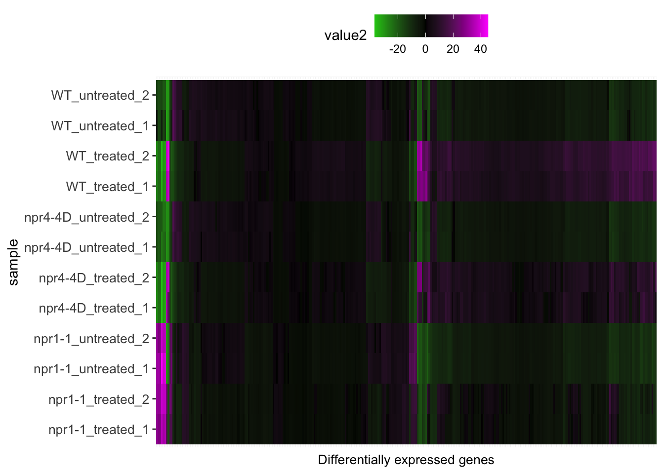
# hide axis ticks and grid lines (error, fix this)
mat <- matrix(unlist(dplyr::select(df,-sample)),nrow=nrow(df))
## Error: Can't subset columns that don't exist.
## [31mx[39m Column `sample` doesn't exist.colnames(mat) <- colnames(df)[1:ncol(df)-1]## Error in colnames(mat) <- colnames(df)[1:ncol(df) - 1]: object 'mat' not foundrownames(mat) <- rownames(df)## Error in rownames(mat) <- rownames(df): object 'mat' not found# hide axis ticks and grid lines
eaxis <- list(
showticklabels = FALSE,
showgrid = FALSE,
zeroline = FALSE
)
p_empty <- plot_ly() %>%
# note that margin applies to entire plot, so we can
# add it here to make tick labels more readable
layout(margin = list(l = 200),
xaxis = eaxis,
yaxis = eaxis)
q1<-subplot(px, p_empty, p, py, nrows = 2, margin = 0.01)## Warning: No trace type specified and no positional attributes specified## No trace type specified:
## Based on info supplied, a 'scatter' trace seems appropriate.
## Read more about this trace type -> https://plotly.com/r/reference/#scatter## No scatter mode specifed:
## Setting the mode to markers
## Read more about this attribute -> https://plotly.com/r/reference/#scatter-mode## Warning: Can only have one: configq1# no gene tree
q2 <- subplot(p,py, nrows = 1, margin = 0.01, widths = c(0.9,0.1), shareX = T,shareY = T)
q2To save image, you need to sign-in plotly website and set environmental variables as described in signup() function help. And then run one line below
plotly_IMAGE(q,width=1000,height=500, format="png",scale=1, out_file=file.path("..","..","..","resources","2018-10-24-dge-clustering-with-ggplot2_files""dendrogram2.png"))More advanced methods
dendextend package Tal Galili (2015), whose updated version can be found in dendextend github.
Session info
sessionInfo()## R version 3.6.2 (2019-12-12)
## Platform: x86_64-apple-darwin15.6.0 (64-bit)
## Running under: macOS Mojave 10.14.6
##
## Matrix products: default
## BLAS: /Library/Frameworks/R.framework/Versions/3.6/Resources/lib/libRblas.0.dylib
## LAPACK: /Library/Frameworks/R.framework/Versions/3.6/Resources/lib/libRlapack.dylib
##
## locale:
## [1] en_US.UTF-8/en_US.UTF-8/en_US.UTF-8/C/en_US.UTF-8/en_US.UTF-8
##
## attached base packages:
## [1] stats graphics grDevices utils datasets methods base
##
## other attached packages:
## [1] edgeR_3.28.1 limma_3.42.2 plotly_4.9.3 ggdendro_0.1.22
## [5] forcats_0.5.0 stringr_1.4.0 dplyr_1.0.2 purrr_0.3.4
## [9] readr_1.4.0 tidyr_1.1.2 tibble_3.0.4 ggplot2_3.3.3
## [13] tidyverse_1.3.0
##
## loaded via a namespace (and not attached):
## [1] Rcpp_1.0.6 locfit_1.5-9.4 lubridate_1.7.9.2 lattice_0.20-41
## [5] assertthat_0.2.1 digest_0.6.27 utf8_1.1.4 R6_2.5.0
## [9] cellranger_1.1.0 backports_1.2.1 reprex_0.3.0 evaluate_0.14
## [13] highr_0.8 httr_1.4.2 blogdown_1.2.2 pillar_1.4.7
## [17] rlang_0.4.10 curl_4.3 lazyeval_0.2.2 readxl_1.3.1
## [21] rstudioapi_0.13 data.table_1.13.6 rmarkdown_2.7 labeling_0.4.2
## [25] htmlwidgets_1.5.3 munsell_0.5.0 broom_0.7.3 compiler_3.6.2
## [29] modelr_0.1.8 xfun_0.22 pkgconfig_2.0.3 htmltools_0.5.1.1
## [33] tidyselect_1.1.0 bookdown_0.21 fansi_0.4.1 viridisLite_0.3.0
## [37] crayon_1.3.4 dbplyr_2.0.0 withr_2.3.0 MASS_7.3-53
## [41] grid_3.6.2 jsonlite_1.7.2 gtable_0.3.0 lifecycle_0.2.0
## [45] DBI_1.1.0 magrittr_2.0.1 scales_1.1.1 cli_2.2.0
## [49] stringi_1.5.3 farver_2.0.3 fs_1.5.0 xml2_1.3.2
## [53] ellipsis_0.3.1 generics_0.1.0 vctrs_0.3.6 tools_3.6.2
## [57] glue_1.4.2 crosstalk_1.1.0.1 hms_0.5.3 yaml_2.2.1
## [61] colorspace_2.0-0 rvest_0.3.6 knitr_1.31 haven_2.3.1