How to draw VennDiagram from differentially expressed genes?
The last time I posted how to draw a VennDiagram with a simulated data. This time I would like to explain how to draw a VennDiagram from differentially expressed genes (DEGs).
Overlap between DEGs from Oct 1, 2018 blog post, “Differential expression analysis with public available sequencing data”
library(limma)
library(tidyverse)
## ── Attaching packages ─────────────────────────────────────── tidyverse 1.3.0 ──## ✓ ggplot2 3.3.3 ✓ purrr 0.3.4
## ✓ tibble 3.0.4 ✓ dplyr 1.0.2
## ✓ tidyr 1.1.2 ✓ stringr 1.4.0
## ✓ readr 1.4.0 ✓ forcats 0.5.0## ── Conflicts ────────────────────────────────────────── tidyverse_conflicts() ──
## x dplyr::filter() masks stats::filter()
## x dplyr::lag() masks stats::lag()# library(ggforce)misregulated geens in npr1-1 in treated samples
load(file.path("..","..","..","resources","2018-12-28-venndiagram-with-differentially-expressed-genes_files","dge.nolow.Ding2018.Rdata"))
dge.nolow
## Loading required package: edgeR## An object of class "DGEList"
## $counts
## SRR6739807 SRR6739808 SRR6739809 SRR6739810 SRR6739811 SRR6739812 SRR6739813
## 1 3598.000 3442.000 3653 3531 4027 3775 4195
## 4 427.000 412.000 316 348 319 357 286
## 5 132.805 129.168 154 141 155 131 126
## 6 52.000 46.000 74 110 122 91 118
## 7 685.000 764.000 231 220 264 247 118
## SRR6739814 SRR6739815 SRR6739816 SRR6739817 SRR6739818
## 1 4317.9900 4015.000 3874.000 3663.000 3642
## 4 306.0000 389.000 362.000 290.000 285
## 5 99.8598 156.895 130.783 101.738 120
## 6 135.0000 60.000 52.000 85.000 79
## 7 131.0000 416.000 383.000 104.000 164
## 16794 more rows ...
##
## $samples
## group lib.size norm.factors Run sample
## SRR6739807 WT_treated 21747803 0.9813040 SRR6739807 WT_treated_1
## SRR6739808 WT_treated 21005249 0.9969243 SRR6739808 WT_treated_2
## SRR6739809 WT_untreated 21052743 0.9901012 SRR6739809 WT_untreated_1
## SRR6739810 WT_untreated 22518666 0.9893923 SRR6739810 WT_untreated_2
## SRR6739811 npr1-1_treated 21437014 1.0185940 SRR6739811 npr1-1_treated_1
## group.1 genotype treatment rep LibraryLayout
## SRR6739807 WT_treated WT treated 1 SINGLE
## SRR6739808 WT_treated WT treated 2 SINGLE
## SRR6739809 WT_untreated WT untreated 1 SINGLE
## SRR6739810 WT_untreated WT untreated 2 SINGLE
## SRR6739811 npr1-1_treated npr1-1 treated 1 SINGLE
## 7 more rows ...
##
## $genes
## genes
## 1 AT1G50920.1
## 4 AT1G15970.1
## 5 AT1G73440.1
## 6 AT1G75120.1
## 7 AT1G17600.1
## 16794 more rows ...# set references in genotype and treatment
dge.nolow$samples$genotype<-factor(dge.nolow$samples$genotype,levels=c("WT","npr4-4D","npr1-1"))
dge.nolow$samples$treatment<-factor(dge.nolow$samples$treatment,levels=c("treated","untreated"))
# making model matrix
design.int <- with(dge.nolow$samples, model.matrix(~ genotype*treatment + rep))
# estimateDisp
dge.nolow.int <- estimateDisp(dge.nolow,design = design.int)
## fit linear model
fit.int <- glmFit(dge.nolow.int,design.int)
# get DEGs, genotype effects in npr1-1 (no matter treated or untreated) (coef=c("genotypenpr1-1","genotypenpr1-1:treatmenttreated"))
genotypenpr1_genotypenpr1.treatmentuntreated.lrt.rWT.rT <- glmLRT(fit.int,coef = c("genotypenpr1-1","genotypenpr1-1:treatmentuntreated"))
genotypenpr1_genotypenpr1.treatmentuntreated.DEGs.int.rWT.rT <- topTags(genotypenpr1_genotypenpr1.treatmentuntreated.lrt.rWT.rT,n = Inf,p.value = 0.05)$table;nrow(genotypenpr1_genotypenpr1.treatmentuntreated.DEGs.int.rWT.rT) # ## [1] 6460Download updated gene description
Most updated annotation can be downloaded from TAIR website (for subscribers). I used “TAIR Data 20180630”. (use donwloaded file. see next chunk)
At.gene.name <-read_tsv("https://www.arabidopsis.org/download_files/Subscriber_Data_Releases/TAIR_Data_20180630/gene_aliases_20180702.txt.gz") # Does work from home when I use Pulse Secure.
# How to concatenate multiple symbols in the same AGI
At.gene.name <- At.gene.name %>% group_by(name) %>% summarise(symbol2=paste(symbol,collapse=";"),full_name=paste(full_name,collapse=";"))
At.gene.name %>% dplyr::slice(100:110) # OK
Using downloaded file (gene_aliases_20201231.txt.gz) (from Differential expression analysis with public available sequencing data, 2018-10-01)
system("gunzip -c ../../../resources/2018-10-01-differential-expression-analysis-with-public-available-sequencing-data_files/gene_aliases_20201231.txt.gz > ../../../resources/2018-10-01-differential-expression-analysis-with-public-available-sequencing-data_files/gene_aliases_20201231.txt")
At.gene.name <- read_tsv(file.path("..","..","..","resources","2018-10-01-differential-expression-analysis-with-public-available-sequencing-data_files","gene_aliases_20201231.txt"))
##
## ── Column specification ────────────────────────────────────────────────────────
## cols(
## name = col_character(),
## symbol = col_character(),
## full_name = col_character()
## )# remove uncompressed file
system("rm ../../../resources/2018-10-01-differential-expression-analysis-with-public-available-sequencing-data_files/gene_aliases_20201231.txt")Add gene descripion to DEG files
# npr1-1 (either treated or untreated)
genotypenpr1_genotypenpr1.treatmentuntreated.DEGs.int.rWT.rT.desc <- genotypenpr1_genotypenpr1.treatmentuntreated.DEGs.int.rWT.rT %>% mutate(AGI=str_remove(genes,pattern="\\.[[:digit:]]+$")) %>% left_join(At.gene.name,by=c("AGI"="name"))
write_csv(genotypenpr1_genotypenpr1.treatmentuntreated.DEGs.int.rWT.rT.desc,file.path("..","..","..","resources","2018-12-28-venndiagram-with-differentially-expressed-genes_files/output/genotypenpr1_genotypenpr1.treatmentuntreated.DEGs.int.rWT.rT.csv"))
read DEG files
# read csv files
getwd()
## [1] "/Volumes/data_personal/Kazu_blog14/content/post/2018-12-28-venndiagram-with-differentially-expressed-genes"## read csv file names
DEG.objs<-list.files(path=file.path("..","..","..","resources","2018-12-28-venndiagram-with-differentially-expressed-genes_files","output"),full.names = TRUE,recursive = TRUE)
DEG.objs## [1] "../../../resources/2018-12-28-venndiagram-with-differentially-expressed-genes_files/output/genotypenpr1_genotypenpr1.treatmenttreated.DEGs.int.rWT.rU.csv"
## [2] "../../../resources/2018-12-28-venndiagram-with-differentially-expressed-genes_files/output/genotypenpr1_genotypenpr1.treatmentuntreated.DEGs.int.rWT.rT.csv"
## [3] "../../../resources/2018-12-28-venndiagram-with-differentially-expressed-genes_files/output/genotypenpr4_genotypenpr4.treatmenttreated.DEGs.int.rWT.rU.csv"
## [4] "../../../resources/2018-12-28-venndiagram-with-differentially-expressed-genes_files/output/trt.DEGs.int.rWT.rU.csv"## read csv files
DEG.count.list <- DEG.objs %>% map(~read_csv(.))##
## ── Column specification ────────────────────────────────────────────────────────
## cols(
## genes = col_character(),
## logFC.genotypenpr1.1 = col_double(),
## logFC.genotypenpr1.1.treatmenttreated = col_double(),
## logCPM = col_double(),
## LR = col_double(),
## PValue = col_double(),
## FDR = col_double(),
## AGI = col_character(),
## symbol2 = col_character(),
## full_name = col_character()
## )##
## ── Column specification ────────────────────────────────────────────────────────
## cols(
## genes = col_character(),
## logFC.genotypenpr1.1 = col_double(),
## logFC.genotypenpr1.1.treatmentuntreated = col_double(),
## logCPM = col_double(),
## LR = col_double(),
## PValue = col_double(),
## FDR = col_double(),
## AGI = col_character(),
## symbol = col_character(),
## full_name = col_character()
## )##
## ── Column specification ────────────────────────────────────────────────────────
## cols(
## genes = col_character(),
## logFC.genotypenpr4.4D = col_double(),
## logFC.genotypenpr4.4D.treatmenttreated = col_double(),
## logCPM = col_double(),
## LR = col_double(),
## PValue = col_double(),
## FDR = col_double(),
## AGI = col_character(),
## symbol2 = col_character(),
## full_name = col_character()
## )##
## ── Column specification ────────────────────────────────────────────────────────
## cols(
## genes = col_character(),
## logFC = col_double(),
## logCPM = col_double(),
## LR = col_double(),
## PValue = col_double(),
## FDR = col_double(),
## AGI = col_character(),
## symbol2 = col_character(),
## full_name = col_character()
## )names(DEG.count.list)<- str_split(DEG.objs,pattern="/",simplify=TRUE)[,7] %>% str_remove(".csv")Interpretation of edgeR glm double coefficient results (topTag)
names(DEG.count.list)## [1] "genotypenpr1_genotypenpr1.treatmenttreated.DEGs.int.rWT.rU"
## [2] "genotypenpr1_genotypenpr1.treatmentuntreated.DEGs.int.rWT.rT"
## [3] "genotypenpr4_genotypenpr4.treatmenttreated.DEGs.int.rWT.rU"
## [4] "trt.DEGs.int.rWT.rU"# reference in treatment was "untreated"
DEG.count.list[["genotypenpr1_genotypenpr1.treatmenttreated.DEGs.int.rWT.rU"]]## # A tibble: 6,460 x 10
## genes logFC.genotypen… logFC.genotypen… logCPM LR PValue FDR
## <chr> <dbl> <dbl> <dbl> <dbl> <dbl> <dbl>
## 1 AT2G… -4.19 -0.733 6.69 1327. 6.75e-289 1.13e-284
## 2 AT5G… 3.26 0.517 4.76 1072. 1.33e-233 1.11e-229
## 3 AT1G… -2.01 -0.488 7.19 659. 6.38e-144 3.57e-140
## 4 AT1G… -2.25 -0.525 7.51 624. 2.54e-136 1.07e-132
## 5 AT3G… -3.15 0.874 5.33 622. 1.00e-135 3.36e-132
## 6 AT5G… -0.206 -6.73 3.90 595. 7.88e-130 2.21e-126
## 7 AT1G… -3.64 -1.53 3.37 581. 7.28e-127 1.75e-123
## 8 AT5G… 1.83 1.82 9.40 571. 1.04e-124 2.18e-121
## 9 AT2G… 2.23 1.94 9.22 559. 4.26e-122 7.94e-119
## 10 AT5G… -2.01 -3.49 4.19 538. 1.19e-117 2.00e-114
## # … with 6,450 more rows, and 3 more variables: AGI <chr>, symbol2 <chr>,
## # full_name <chr># reference in treatment was "treated"
## genotypenpr1_genotypenpr1.treatmentuntreated.DEGs.int.rWT.rT
DEG.count.list[["genotypenpr1_genotypenpr1.treatmentuntreated.DEGs.int.rWT.rT"]]## # A tibble: 10,074 x 10
## genes logFC.genotypen… logFC.genotypen… logCPM LR PValue FDR
## <chr> <dbl> <dbl> <dbl> <dbl> <dbl> <dbl>
## 1 AT2G… -4.92 0.733 6.69 1327. 6.75e-289 1.13e-284
## 2 AT5G… 3.78 -0.517 4.76 1072. 1.33e-233 1.11e-229
## 3 AT1G… -2.50 0.488 7.19 659. 6.38e-144 3.57e-140
## 4 AT1G… -2.50 0.488 7.19 659. 6.38e-144 3.57e-140
## 5 AT1G… -2.50 0.488 7.19 659. 6.38e-144 3.57e-140
## 6 AT1G… -2.78 0.525 7.51 624. 2.54e-136 1.07e-132
## 7 AT3G… -2.28 -0.874 5.33 622. 1.00e-135 3.36e-132
## 8 AT5G… -6.94 6.73 3.90 595. 7.88e-130 2.21e-126
## 9 AT5G… -6.94 6.73 3.90 595. 7.88e-130 2.21e-126
## 10 AT5G… -6.94 6.73 3.90 595. 7.88e-130 2.21e-126
## # … with 10,064 more rows, and 3 more variables: AGI <chr>, symbol <chr>,
## # full_name <chr># Total numbe of DEGS are the same off course.
# Absolute value of "logFC.genotypenpr1.1.treatmenttreated" in genotypenpr1_genotypenpr1.treatmenttreated.DEGs.int.rWT.rU.csv is the same with one in "logFC.genotypenpr1.1.treatmentuntreated" in genotypenpr1_genotypenpr1.treatmentuntreated.DEGs.int.rWT.rT.csv and only signs (positive or negative) are different.
# logFC.genotypenpr1.1 column
## In "genotypenpr1_genotypenpr1.treatmentuntreated.DEGs.int.rWT.rT.csv", logFC value are calculated for "treated" (=reference is "treated"; rT) samples.
## In "genotypenpr1_genotypenpr1.treatmenttreated.DEGs.int.rWT.rU.csv", logFC value are calculated for "treated" (=reference is "treated"; rT) samples.making summary table
# combine all DEG gene names
all.DEGs<-unique(c(DEG.count.list[["genotypenpr1_genotypenpr1.treatmenttreated.DEGs.int.rWT.rU"]]$genes,DEG.count.list[["trt.DEGs.int.rWT.rU"]]$genes))
#
WT.SA.up<-DEG.count.list[["trt.DEGs.int.rWT.rU"]] %>% filter(logFC>0) %>% mutate(WT.SA.up=1) %>% select(genes,WT.SA.up)
WT.SA.down<-DEG.count.list[["trt.DEGs.int.rWT.rU"]] %>% filter(logFC<0) %>% mutate(WT.SA.down=1) %>% select(genes,WT.SA.down)
# npr1.1 regulated genes
npr1.gt<-DEG.count.list[["genotypenpr1_genotypenpr1.treatmenttreated.DEGs.int.rWT.rU"]] %>% mutate(npr1.gt=1) %>% select(genes,npr1.gt)

# summarize
summary.DEGS<-tibble(genes=all.DEGs) %>% full_join(WT.SA.up,by="genes") %>% full_join(WT.SA.down,by="genes") %>% full_join(npr1.gt,by="genes")
dim(summary.DEGS)[1]==length(all.DEGs)
## [1] TRUEsummary.DEGS[is.na(summary.DEGS)]<-0
# convert into count table
vdc<-limma::vennCounts(summary.DEGS[,-1])
# plot (classical way)
limma::vennDiagram(vdc) # traditional version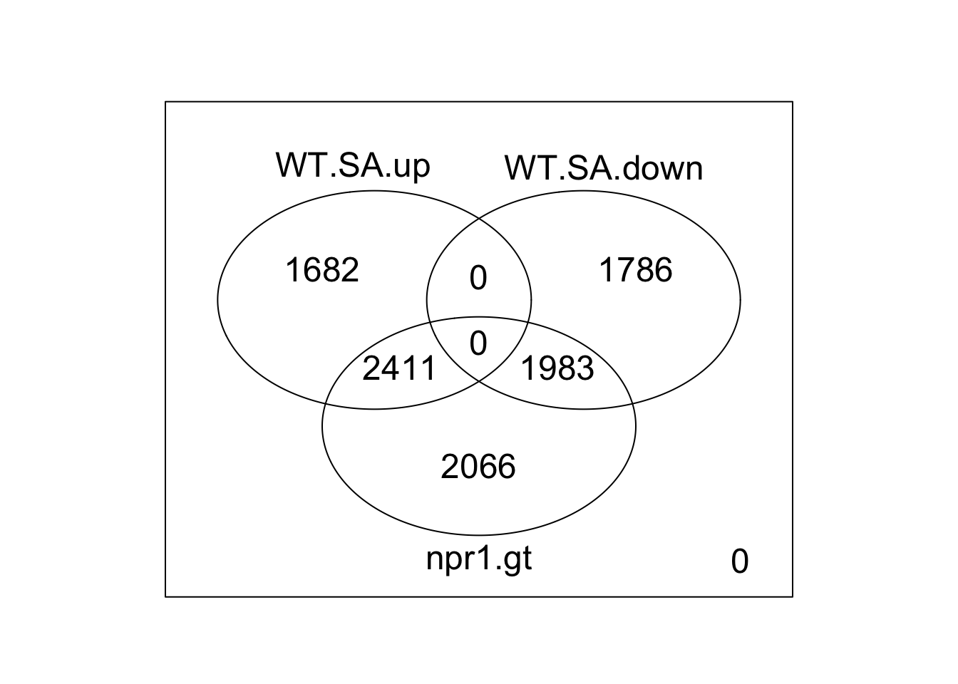
# plot (ggplot2 version) ### under construction ####Session info
sessionInfo()## R version 3.6.2 (2019-12-12)
## Platform: x86_64-apple-darwin15.6.0 (64-bit)
## Running under: macOS Mojave 10.14.6
##
## Matrix products: default
## BLAS: /Library/Frameworks/R.framework/Versions/3.6/Resources/lib/libRblas.0.dylib
## LAPACK: /Library/Frameworks/R.framework/Versions/3.6/Resources/lib/libRlapack.dylib
##
## locale:
## [1] en_US.UTF-8/en_US.UTF-8/en_US.UTF-8/C/en_US.UTF-8/en_US.UTF-8
##
## attached base packages:
## [1] stats graphics grDevices utils datasets methods base
##
## other attached packages:
## [1] edgeR_3.28.1 forcats_0.5.0 stringr_1.4.0 dplyr_1.0.2
## [5] purrr_0.3.4 readr_1.4.0 tidyr_1.1.2 tibble_3.0.4
## [9] ggplot2_3.3.3 tidyverse_1.3.0 limma_3.42.2
##
## loaded via a namespace (and not attached):
## [1] locfit_1.5-9.4 tidyselect_1.1.0 xfun_0.22 splines_3.6.2
## [5] lattice_0.20-41 haven_2.3.1 colorspace_2.0-0 vctrs_0.3.6
## [9] generics_0.1.0 htmltools_0.5.1.1 yaml_2.2.1 utf8_1.1.4
## [13] rlang_0.4.10 pillar_1.4.7 glue_1.4.2 withr_2.3.0
## [17] DBI_1.1.0 dbplyr_2.0.0 modelr_0.1.8 readxl_1.3.1
## [21] lifecycle_0.2.0 munsell_0.5.0 blogdown_1.2.2 gtable_0.3.0
## [25] cellranger_1.1.0 rvest_0.3.6 evaluate_0.14 knitr_1.31
## [29] fansi_0.4.1 highr_0.8 broom_0.7.3 Rcpp_1.0.6
## [33] scales_1.1.1 backports_1.2.1 jsonlite_1.7.2 fs_1.5.0
## [37] hms_0.5.3 digest_0.6.27 stringi_1.5.3 bookdown_0.21
## [41] grid_3.6.2 cli_2.2.0 tools_3.6.2 magrittr_2.0.1
## [45] crayon_1.3.4 pkgconfig_2.0.3 ellipsis_0.3.1 xml2_1.3.2
## [49] reprex_0.3.0 lubridate_1.7.9.2 assertthat_0.2.1 rmarkdown_2.7
## [53] httr_1.4.2 rstudioapi_0.13 R6_2.5.0 compiler_3.6.2