Useful R techniques (only for me?)
Usage of filter()
mtcars %>% rownames_to_column() %>% filter(str_detect(rowname,"Mazda"))## rowname mpg cyl disp hp drat wt qsec vs am gear carb
## 1 Mazda RX4 21 6 160 110 3.9 2.620 16.46 0 1 4 4
## 2 Mazda RX4 Wag 21 6 160 110 3.9 2.875 17.02 0 1 4 4mtcars %>% rownames_to_column() %>% filter(!str_detect(rowname,"Mazda"))## rowname mpg cyl disp hp drat wt qsec vs am gear carb
## 1 Datsun 710 22.8 4 108.0 93 3.85 2.320 18.61 1 1 4 1
## 2 Hornet 4 Drive 21.4 6 258.0 110 3.08 3.215 19.44 1 0 3 1
## 3 Hornet Sportabout 18.7 8 360.0 175 3.15 3.440 17.02 0 0 3 2
## 4 Valiant 18.1 6 225.0 105 2.76 3.460 20.22 1 0 3 1
## 5 Duster 360 14.3 8 360.0 245 3.21 3.570 15.84 0 0 3 4
## 6 Merc 240D 24.4 4 146.7 62 3.69 3.190 20.00 1 0 4 2
## 7 Merc 230 22.8 4 140.8 95 3.92 3.150 22.90 1 0 4 2
## 8 Merc 280 19.2 6 167.6 123 3.92 3.440 18.30 1 0 4 4
## 9 Merc 280C 17.8 6 167.6 123 3.92 3.440 18.90 1 0 4 4
## 10 Merc 450SE 16.4 8 275.8 180 3.07 4.070 17.40 0 0 3 3
## 11 Merc 450SL 17.3 8 275.8 180 3.07 3.730 17.60 0 0 3 3
## 12 Merc 450SLC 15.2 8 275.8 180 3.07 3.780 18.00 0 0 3 3
## 13 Cadillac Fleetwood 10.4 8 472.0 205 2.93 5.250 17.98 0 0 3 4
## 14 Lincoln Continental 10.4 8 460.0 215 3.00 5.424 17.82 0 0 3 4
## 15 Chrysler Imperial 14.7 8 440.0 230 3.23 5.345 17.42 0 0 3 4
## 16 Fiat 128 32.4 4 78.7 66 4.08 2.200 19.47 1 1 4 1
## 17 Honda Civic 30.4 4 75.7 52 4.93 1.615 18.52 1 1 4 2
## 18 Toyota Corolla 33.9 4 71.1 65 4.22 1.835 19.90 1 1 4 1
## 19 Toyota Corona 21.5 4 120.1 97 3.70 2.465 20.01 1 0 3 1
## 20 Dodge Challenger 15.5 8 318.0 150 2.76 3.520 16.87 0 0 3 2
## 21 AMC Javelin 15.2 8 304.0 150 3.15 3.435 17.30 0 0 3 2
## 22 Camaro Z28 13.3 8 350.0 245 3.73 3.840 15.41 0 0 3 4
## 23 Pontiac Firebird 19.2 8 400.0 175 3.08 3.845 17.05 0 0 3 2
## 24 Fiat X1-9 27.3 4 79.0 66 4.08 1.935 18.90 1 1 4 1
## 25 Porsche 914-2 26.0 4 120.3 91 4.43 2.140 16.70 0 1 5 2
## 26 Lotus Europa 30.4 4 95.1 113 3.77 1.513 16.90 1 1 5 2
## 27 Ford Pantera L 15.8 8 351.0 264 4.22 3.170 14.50 0 1 5 4
## 28 Ferrari Dino 19.7 6 145.0 175 3.62 2.770 15.50 0 1 5 6
## 29 Maserati Bora 15.0 8 301.0 335 3.54 3.570 14.60 0 1 5 8
## 30 Volvo 142E 21.4 4 121.0 109 4.11 2.780 18.60 1 1 4 2mtcars %>% rownames_to_column() %>% filter(str_detect(rowname,"[:alphabet:]+")) # error## Error: Problem with `filter()` input `..1`.
## x Start of codes indicating failure. (U_ILLEGAL_ARGUMENT_ERROR)
## ℹ Input `..1` is `str_detect(rowname, "[:alphabet:]+")`.Applying map() to list object by using split()
- Look “Unquoting” for as.name()
scatter_by2 <- function(data, x, y) {
#print("x is")
# print(x) # error
  x <- enquo(x)
print("x is");print(x)
print("y is");print(y)
print("aes(!!x, !!y) is "); print(aes(!!x, !!y))
  ggplot(data) + geom_point(aes(!!x, !!y))
}
scatter_by2(mtcars, disp, "drat") # does not work
## [1] "x is"
## <quosure>
## expr: ^disp
## env: global
## [1] "y is"
## [1] "drat"
## [1] "aes(!!x, !!y) is "
## Aesthetic mapping:
## * `x` -> `disp`
## * `y` -> "drat"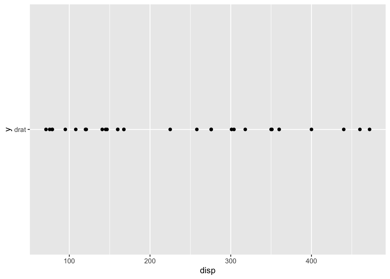
input <- as.name("drat")
scatter_by2(mtcars, disp, input) # does  work
## [1] "x is"
## <quosure>
## expr: ^disp
## env: global
## [1] "y is"
## drat
## [1] "aes(!!x, !!y) is "
## Aesthetic mapping:
## * `x` -> `disp`
## * `y` -> `drat`
scatter_by2(mtcars, disp, as.name("drat")) # does work## [1] "x is"
## <quosure>
## expr: ^disp
## env: global
## [1] "y is"
## drat
## [1] "aes(!!x, !!y) is "
## Aesthetic mapping:
## * `x` -> `disp`
## * `y` -> `drat`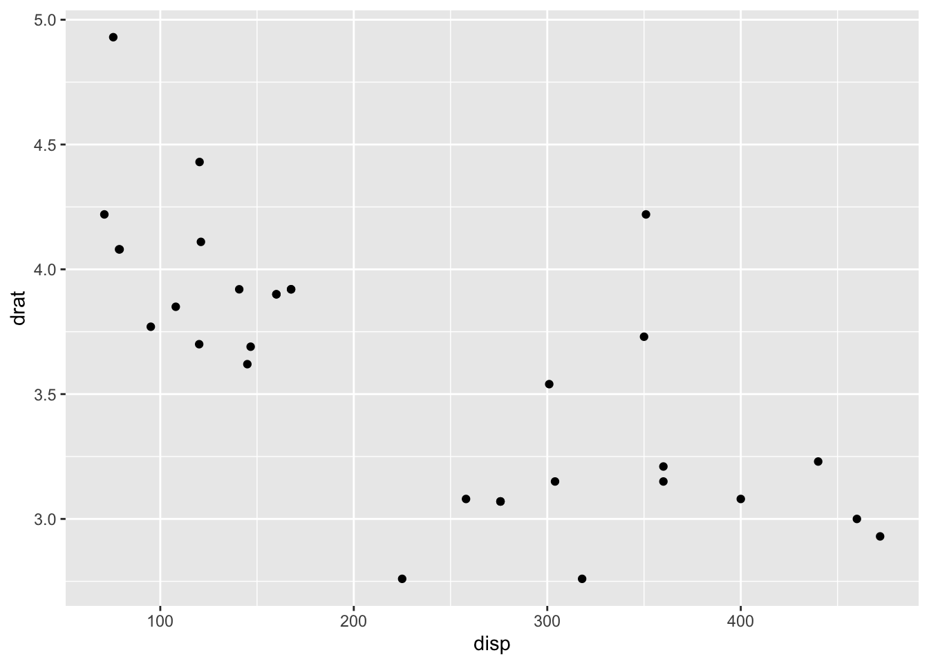
parameters <- names(mtcars)
plot.list <- tibble(parameters=names(mtcars)) %>% split(.$parameters) %>% map(~scatter_by2(mtcars, disp, as.name(.$parameters)))
## [1] "x is"
## <quosure>
## expr: ^disp
## env: 0x7f81ae6435d0
## [1] "y is"
## am
## [1] "aes(!!x, !!y) is "
## Aesthetic mapping:
## * `x` -> `disp`
## * `y` -> `am`
## [1] "x is"
## <quosure>
## expr: ^disp
## env: 0x7f81adc10d58
## [1] "y is"
## carb
## [1] "aes(!!x, !!y) is "
## Aesthetic mapping:
## * `x` -> `disp`
## * `y` -> `carb`
## [1] "x is"
## <quosure>
## expr: ^disp
## env: 0x7f81abfb5ff0
## [1] "y is"
## cyl
## [1] "aes(!!x, !!y) is "
## Aesthetic mapping:
## * `x` -> `disp`
## * `y` -> `cyl`
## [1] "x is"
## <quosure>
## expr: ^disp
## env: 0x7f81ab8d3758
## [1] "y is"
## disp
## [1] "aes(!!x, !!y) is "
## Aesthetic mapping:
## * `x` -> `disp`
## * `y` -> `disp`
## [1] "x is"
## <quosure>
## expr: ^disp
## env: 0x7f81b20f9d00
## [1] "y is"
## drat
## [1] "aes(!!x, !!y) is "
## Aesthetic mapping:
## * `x` -> `disp`
## * `y` -> `drat`
## [1] "x is"
## <quosure>
## expr: ^disp
## env: 0x7f81b21b14e8
## [1] "y is"
## gear
## [1] "aes(!!x, !!y) is "
## Aesthetic mapping:
## * `x` -> `disp`
## * `y` -> `gear`
## [1] "x is"
## <quosure>
## expr: ^disp
## env: 0x7f81b0694158
## [1] "y is"
## hp
## [1] "aes(!!x, !!y) is "
## Aesthetic mapping:
## * `x` -> `disp`
## * `y` -> `hp`
## [1] "x is"
## <quosure>
## expr: ^disp
## env: 0x7f81b231fac0
## [1] "y is"
## mpg
## [1] "aes(!!x, !!y) is "
## Aesthetic mapping:
## * `x` -> `disp`
## * `y` -> `mpg`
## [1] "x is"
## <quosure>
## expr: ^disp
## env: 0x7f81b0af47c8
## [1] "y is"
## qsec
## [1] "aes(!!x, !!y) is "
## Aesthetic mapping:
## * `x` -> `disp`
## * `y` -> `qsec`
## [1] "x is"
## <quosure>
## expr: ^disp
## env: 0x7f81b128ca20
## [1] "y is"
## vs
## [1] "aes(!!x, !!y) is "
## Aesthetic mapping:
## * `x` -> `disp`
## * `y` -> `vs`
## [1] "x is"
## <quosure>
## expr: ^disp
## env: 0x7f81b07a7f38
## [1] "y is"
## wt
## [1] "aes(!!x, !!y) is "
## Aesthetic mapping:
## * `x` -> `disp`
## * `y` -> `wt`plot.list[[1]]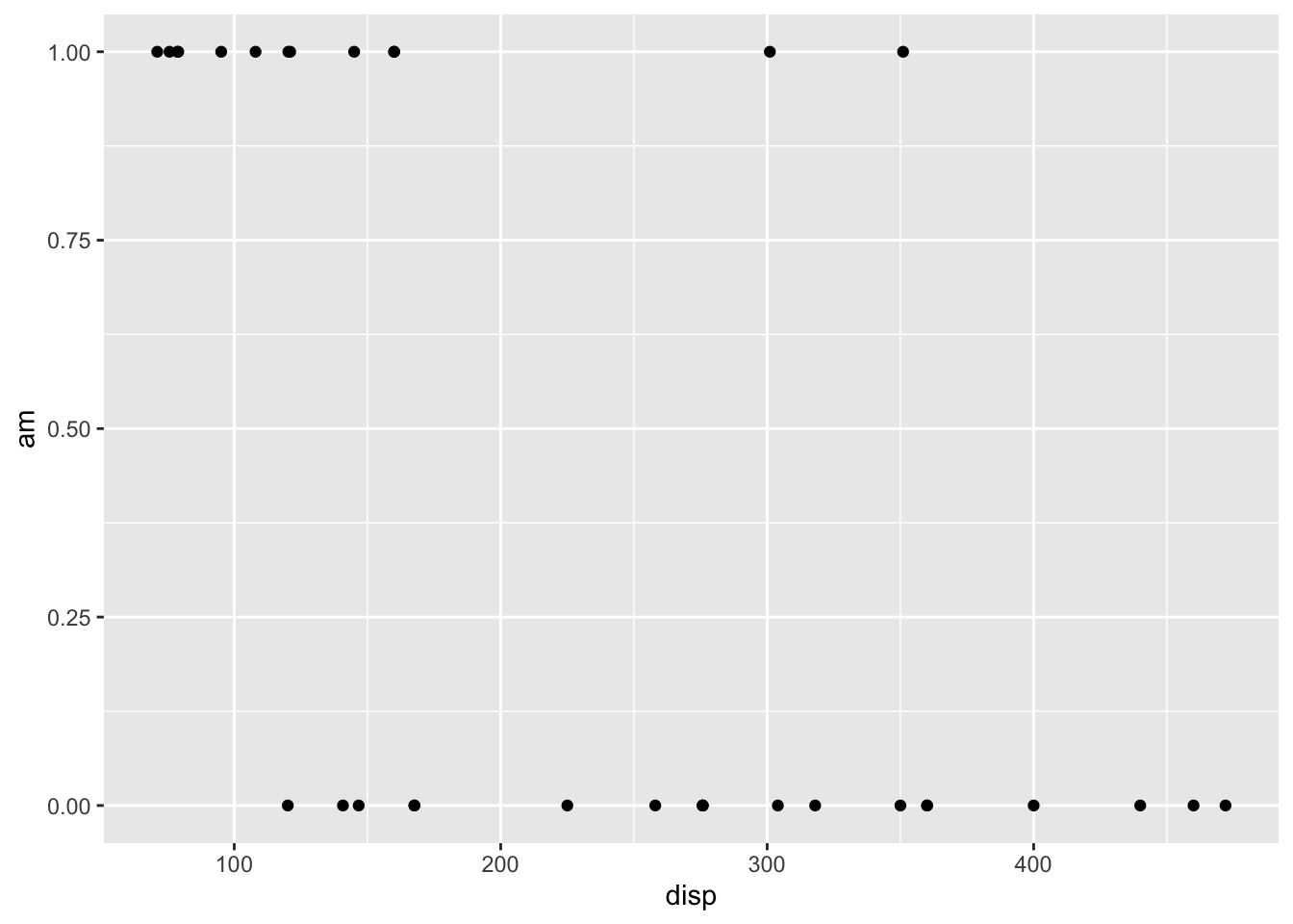
plot.list[[2]]
plot.list[[3]]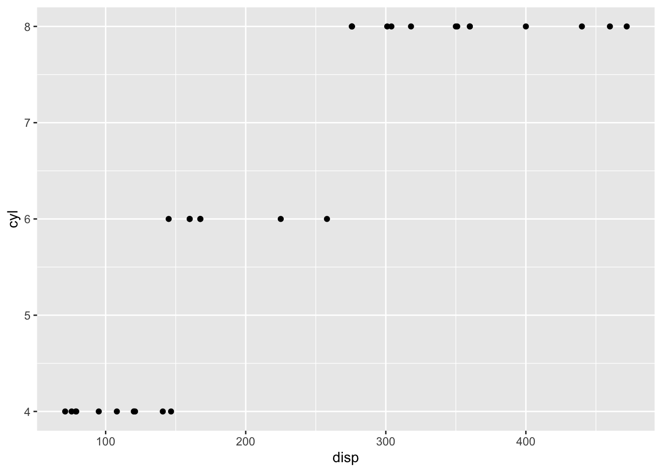
sample data
custom.categoreis.map <- c(
  "cold_Kilian_2007.root.fits.summary.AGI.FC.csv.gz",
  "cold_Kilian_2007.shoot.fits.summary.AGI.FC.csv.gz",
  "Fe_def_KIM_2019_pnas.1916892116.sd01.csv",
  "Heat_Kilian_2007.root.fits.summary.AGI.FC.csv.gz",
  "Heat_Kilian_2007.shoot.fits.summary.AGI.FC.csv.gz",
  "minusB_Nishida_2017_root.DEGs.csv.gz",
  "minusCa_Nishida_2017_root.DEGs.csv.gz",
  "minusCu_Nishida_2017_root.DEGs.csv.gz",
  "minusFe_Kailasam2019.DEGs.all.anno.csv.gz",
  "minusFe_Kim2019.fits.summary.AGI.FC.WT.csv.gz",
  "minusFe_Kim2019.fits.summary.locus.FC.WT.csv.gz",
  "minusFe_Nishida_2017_root.DEGs.csv.gz",
  "minusK_Nishida_2017_root.DEGs.csv.gz",
  "minusMg_Nishida_2017_root.DEGs.csv.gz",
  "minusMg_Niu_2016_root.DEGs.csv.gz",
  "minusMg_Niu_2016_shoot.DEGs.csv.gz",
  "minusMn_Nishida_2017_root.DEGs.csv.gz",
  "minusMn_Rodriguez-Celma_2016.DEGs.all.anno.csv.gz",
  "minusMo_Nishida_2017_root.DEGs.csv.gz",
  "minusN_Gutierrez_2007.root.fits.summary.AGI.FC.csv.gz",
  "minusN_Nishida_2017_root.DEGs.csv.gz",
  "minusN_Peng_2007.AGI.FC.csv.gz",
  "minusN_Peng_2007.Br.FC.csv.gz",
  "minusP_Nishida_2017_root.DEGs.csv.gz",
  "minusPi_1d_Liu_2016_root.DEGs.csv.gz",
  "minusPi_1d_Liu_2016_shoot.DEGs.csv.gz",
  "minusPi_3d_Liu_2016_root.DEGs.csv.gz",
  "minusPi_3d_Liu_2016_shoot.DEGs.csv.gz",
  "minusS_Aarabi2016.fits.summary.AGI.FC.csv.gz",
  "minusS_Nishida_2017_root.DEGs.csv.gz",
  "minusZn_Nishida_2017_root.DEGs.csv.gz",
  "plusAl_Ligaba-OSena_2017_root.DEGs.csv.gz",
  "plusAl_Ligaba-OSena_2017_shoot.DEGs.csv.gz",
  "plusIAA_Nemhauser_2006_seedlings.AGI.FC.csv.gz",
  "plusIAA_Nemhauser_2006_seedlings.Br.FC.csv.gz",
  "plusMg_Niu_2016_root.DEGs.csv.gz",
  "plusMg_Niu_2016_shoot.DEGs.csv.gz",
  "plusN_Wang2003.root.fits.summary.AGI.FC.csv.gz",
  "plusN_Wang2003.shoot.fits.summary.AGI.FC.csv.gz")
To extract Nishida’s DEGs, grep(value=TRUE) can be used for classic R.
custom.categoreis.map %>% grep(pattern="Nishida",value=TRUE)## [1] "minusB_Nishida_2017_root.DEGs.csv.gz"
## [2] "minusCa_Nishida_2017_root.DEGs.csv.gz"
## [3] "minusCu_Nishida_2017_root.DEGs.csv.gz"
## [4] "minusFe_Nishida_2017_root.DEGs.csv.gz"
## [5] "minusK_Nishida_2017_root.DEGs.csv.gz"
## [6] "minusMg_Nishida_2017_root.DEGs.csv.gz"
## [7] "minusMn_Nishida_2017_root.DEGs.csv.gz"
## [8] "minusMo_Nishida_2017_root.DEGs.csv.gz"
## [9] "minusN_Nishida_2017_root.DEGs.csv.gz"
## [10] "minusP_Nishida_2017_root.DEGs.csv.gz"
## [11] "minusS_Nishida_2017_root.DEGs.csv.gz"
## [12] "minusZn_Nishida_2017_root.DEGs.csv.gz"The tidyverse way is using str_subset().
custom.categoreis.map %>% str_subset("Nishida")## [1] "minusB_Nishida_2017_root.DEGs.csv.gz"
## [2] "minusCa_Nishida_2017_root.DEGs.csv.gz"
## [3] "minusCu_Nishida_2017_root.DEGs.csv.gz"
## [4] "minusFe_Nishida_2017_root.DEGs.csv.gz"
## [5] "minusK_Nishida_2017_root.DEGs.csv.gz"
## [6] "minusMg_Nishida_2017_root.DEGs.csv.gz"
## [7] "minusMn_Nishida_2017_root.DEGs.csv.gz"
## [8] "minusMo_Nishida_2017_root.DEGs.csv.gz"
## [9] "minusN_Nishida_2017_root.DEGs.csv.gz"
## [10] "minusP_Nishida_2017_root.DEGs.csv.gz"
## [11] "minusS_Nishida_2017_root.DEGs.csv.gz"
## [12] "minusZn_Nishida_2017_root.DEGs.csv.gz"Other than “Nishida”. (classic R version)
custom.categoreis.map %>% grep(pattern="Nishida",value=TRUE,invert=TRUE)## [1] "cold_Kilian_2007.root.fits.summary.AGI.FC.csv.gz"
## [2] "cold_Kilian_2007.shoot.fits.summary.AGI.FC.csv.gz"
## [3] "Fe_def_KIM_2019_pnas.1916892116.sd01.csv"
## [4] "Heat_Kilian_2007.root.fits.summary.AGI.FC.csv.gz"
## [5] "Heat_Kilian_2007.shoot.fits.summary.AGI.FC.csv.gz"
## [6] "minusFe_Kailasam2019.DEGs.all.anno.csv.gz"
## [7] "minusFe_Kim2019.fits.summary.AGI.FC.WT.csv.gz"
## [8] "minusFe_Kim2019.fits.summary.locus.FC.WT.csv.gz"
## [9] "minusMg_Niu_2016_root.DEGs.csv.gz"
## [10] "minusMg_Niu_2016_shoot.DEGs.csv.gz"
## [11] "minusMn_Rodriguez-Celma_2016.DEGs.all.anno.csv.gz"
## [12] "minusN_Gutierrez_2007.root.fits.summary.AGI.FC.csv.gz"
## [13] "minusN_Peng_2007.AGI.FC.csv.gz"
## [14] "minusN_Peng_2007.Br.FC.csv.gz"
## [15] "minusPi_1d_Liu_2016_root.DEGs.csv.gz"
## [16] "minusPi_1d_Liu_2016_shoot.DEGs.csv.gz"
## [17] "minusPi_3d_Liu_2016_root.DEGs.csv.gz"
## [18] "minusPi_3d_Liu_2016_shoot.DEGs.csv.gz"
## [19] "minusS_Aarabi2016.fits.summary.AGI.FC.csv.gz"
## [20] "plusAl_Ligaba-OSena_2017_root.DEGs.csv.gz"
## [21] "plusAl_Ligaba-OSena_2017_shoot.DEGs.csv.gz"
## [22] "plusIAA_Nemhauser_2006_seedlings.AGI.FC.csv.gz"
## [23] "plusIAA_Nemhauser_2006_seedlings.Br.FC.csv.gz"
## [24] "plusMg_Niu_2016_root.DEGs.csv.gz"
## [25] "plusMg_Niu_2016_shoot.DEGs.csv.gz"
## [26] "plusN_Wang2003.root.fits.summary.AGI.FC.csv.gz"
## [27] "plusN_Wang2003.shoot.fits.summary.AGI.FC.csv.gz"Other than “Nishida”. (tidyverse version)
custom.categoreis.map %>% str_subset("Nishida",negate=TRUE)## [1] "cold_Kilian_2007.root.fits.summary.AGI.FC.csv.gz"
## [2] "cold_Kilian_2007.shoot.fits.summary.AGI.FC.csv.gz"
## [3] "Fe_def_KIM_2019_pnas.1916892116.sd01.csv"
## [4] "Heat_Kilian_2007.root.fits.summary.AGI.FC.csv.gz"
## [5] "Heat_Kilian_2007.shoot.fits.summary.AGI.FC.csv.gz"
## [6] "minusFe_Kailasam2019.DEGs.all.anno.csv.gz"
## [7] "minusFe_Kim2019.fits.summary.AGI.FC.WT.csv.gz"
## [8] "minusFe_Kim2019.fits.summary.locus.FC.WT.csv.gz"
## [9] "minusMg_Niu_2016_root.DEGs.csv.gz"
## [10] "minusMg_Niu_2016_shoot.DEGs.csv.gz"
## [11] "minusMn_Rodriguez-Celma_2016.DEGs.all.anno.csv.gz"
## [12] "minusN_Gutierrez_2007.root.fits.summary.AGI.FC.csv.gz"
## [13] "minusN_Peng_2007.AGI.FC.csv.gz"
## [14] "minusN_Peng_2007.Br.FC.csv.gz"
## [15] "minusPi_1d_Liu_2016_root.DEGs.csv.gz"
## [16] "minusPi_1d_Liu_2016_shoot.DEGs.csv.gz"
## [17] "minusPi_3d_Liu_2016_root.DEGs.csv.gz"
## [18] "minusPi_3d_Liu_2016_shoot.DEGs.csv.gz"
## [19] "minusS_Aarabi2016.fits.summary.AGI.FC.csv.gz"
## [20] "plusAl_Ligaba-OSena_2017_root.DEGs.csv.gz"
## [21] "plusAl_Ligaba-OSena_2017_shoot.DEGs.csv.gz"
## [22] "plusIAA_Nemhauser_2006_seedlings.AGI.FC.csv.gz"
## [23] "plusIAA_Nemhauser_2006_seedlings.Br.FC.csv.gz"
## [24] "plusMg_Niu_2016_root.DEGs.csv.gz"
## [25] "plusMg_Niu_2016_shoot.DEGs.csv.gz"
## [26] "plusN_Wang2003.root.fits.summary.AGI.FC.csv.gz"
## [27] "plusN_Wang2003.shoot.fits.summary.AGI.FC.csv.gz"ggplot legend size
df <- expand.grid(X1 = 1:10, X2 = 1:10)
df$value <- df$X1 * df$X2

p1 <- ggplot(df, aes(X1, X2)) + geom_tile(aes(fill = value))
p2 <- p1 + geom_point(aes(size = value))
p2 + theme(legend.key.size= unit(2, "cm"))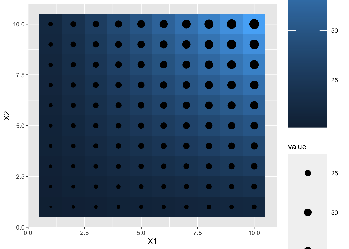
p2 + theme(legend.key.width= unit(2, "cm"))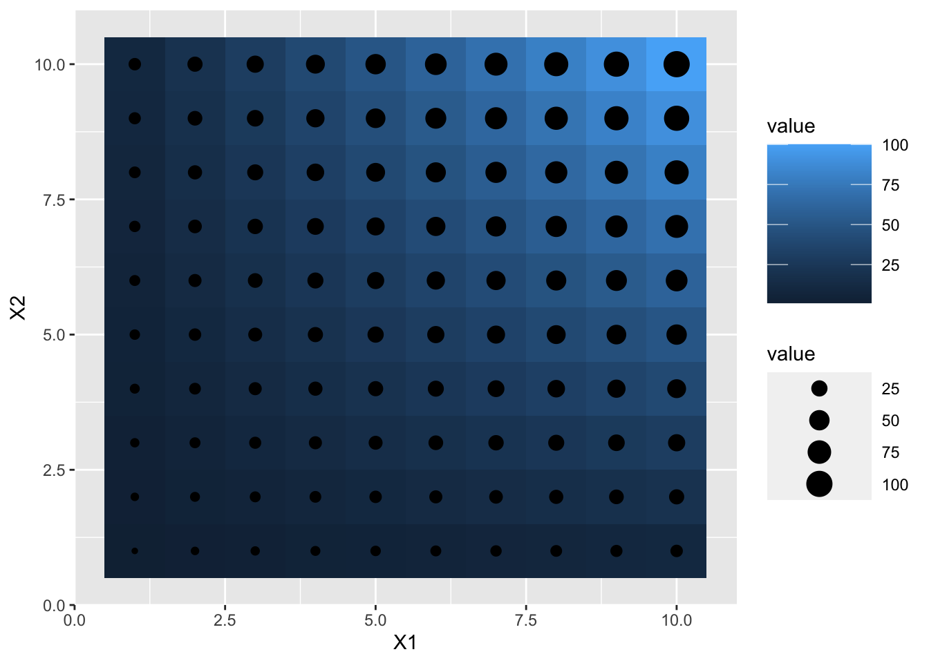
p2 + theme(legend.key.height= unit(2, "cm"))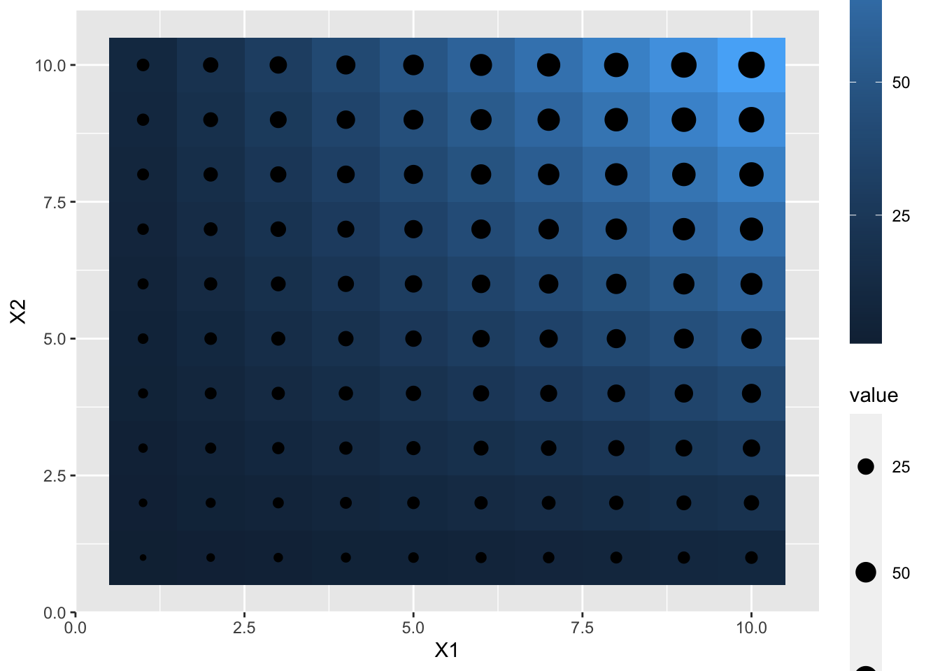
pivot_longer, pivot_wider
- Those are cited from
vignette("pivot")## starting httpd help server ... done- The dataset (“relig_income”) contains three variables: religion, stored in the rows, income spread across the column names, and count stored in the cell values.
- To tidy it we use pivot_longer():
relig_income## # A tibble: 18 x 11
## religion `<$10k` `$10-20k` `$20-30k` `$30-40k` `$40-50k` `$50-75k` `$75-100k`
## <chr> <dbl> <dbl> <dbl> <dbl> <dbl> <dbl> <dbl>
## 1 Agnostic 27 34 60 81 76 137 122
## 2 Atheist 12 27 37 52 35 70 73
## 3 Buddhist 27 21 30 34 33 58 62
## 4 Catholic 418 617 732 670 638 1116 949
## 5 Don’t k… 15 14 15 11 10 35 21
## 6 Evangel… 575 869 1064 982 881 1486 949
## 7 Hindu 1 9 7 9 11 34 47
## 8 Histori… 228 244 236 238 197 223 131
## 9 Jehovah… 20 27 24 24 21 30 15
## 10 Jewish 19 19 25 25 30 95 69
## 11 Mainlin… 289 495 619 655 651 1107 939
## 12 Mormon 29 40 48 51 56 112 85
## 13 Muslim 6 7 9 10 9 23 16
## 14 Orthodox 13 17 23 32 32 47 38
## 15 Other C… 9 7 11 13 13 14 18
## 16 Other F… 20 33 40 46 49 63 46
## 17 Other W… 5 2 3 4 2 7 3
## 18 Unaffil… 217 299 374 365 341 528 407
## # … with 3 more variables: `$100-150k` <dbl>, `>150k` <dbl>, `Don't
## # know/refused` <dbl>relig_income %>% pivot_longer(-religion, names_to = "income", values_to = "count")## # A tibble: 180 x 3
## religion income count
## <chr> <chr> <dbl>
## 1 Agnostic <$10k 27
## 2 Agnostic $10-20k 34
## 3 Agnostic $20-30k 60
## 4 Agnostic $30-40k 81
## 5 Agnostic $40-50k 76
## 6 Agnostic $50-75k 137
## 7 Agnostic $75-100k 122
## 8 Agnostic $100-150k 109
## 9 Agnostic >150k 84
## 10 Agnostic Don't know/refused 96
## # … with 170 more rowsThe first argument is the dataset to reshape, relig_income.
The second argument describes which columns need to be reshaped. In this case, it’s every column apart from religion.
The names_to gives the name of the variable that will be created from the data stored in the column names, i.e. income.
The values_to gives the name of the variable that will be created from the data stored in the cell value, i.e. count.
Neither the names_to nor the values_to column exists in relig_income, so we provide them as character strings surrounded in quotes.
Numeric data in column names
billboard## # A tibble: 317 x 79
## artist track date.entered wk1 wk2 wk3 wk4 wk5 wk6 wk7 wk8
## <chr> <chr> <date> <dbl> <dbl> <dbl> <dbl> <dbl> <dbl> <dbl> <dbl>
## 1 2 Pac Baby… 2000-02-26 87 82 72 77 87 94 99 NA
## 2 2Ge+h… The … 2000-09-02 91 87 92 NA NA NA NA NA
## 3 3 Doo… Kryp… 2000-04-08 81 70 68 67 66 57 54 53
## 4 3 Doo… Loser 2000-10-21 76 76 72 69 67 65 55 59
## 5 504 B… Wobb… 2000-04-15 57 34 25 17 17 31 36 49
## 6 98^0 Give… 2000-08-19 51 39 34 26 26 19 2 2
## 7 A*Tee… Danc… 2000-07-08 97 97 96 95 100 NA NA NA
## 8 Aaliy… I Do… 2000-01-29 84 62 51 41 38 35 35 38
## 9 Aaliy… Try … 2000-03-18 59 53 38 28 21 18 16 14
## 10 Adams… Open… 2000-08-26 76 76 74 69 68 67 61 58
## # … with 307 more rows, and 68 more variables: wk9 <dbl>, wk10 <dbl>,
## # wk11 <dbl>, wk12 <dbl>, wk13 <dbl>, wk14 <dbl>, wk15 <dbl>, wk16 <dbl>,
## # wk17 <dbl>, wk18 <dbl>, wk19 <dbl>, wk20 <dbl>, wk21 <dbl>, wk22 <dbl>,
## # wk23 <dbl>, wk24 <dbl>, wk25 <dbl>, wk26 <dbl>, wk27 <dbl>, wk28 <dbl>,
## # wk29 <dbl>, wk30 <dbl>, wk31 <dbl>, wk32 <dbl>, wk33 <dbl>, wk34 <dbl>,
## # wk35 <dbl>, wk36 <dbl>, wk37 <dbl>, wk38 <dbl>, wk39 <dbl>, wk40 <dbl>,
## # wk41 <dbl>, wk42 <dbl>, wk43 <dbl>, wk44 <dbl>, wk45 <dbl>, wk46 <dbl>,
## # wk47 <dbl>, wk48 <dbl>, wk49 <dbl>, wk50 <dbl>, wk51 <dbl>, wk52 <dbl>,
## # wk53 <dbl>, wk54 <dbl>, wk55 <dbl>, wk56 <dbl>, wk57 <dbl>, wk58 <dbl>,
## # wk59 <dbl>, wk60 <dbl>, wk61 <dbl>, wk62 <dbl>, wk63 <dbl>, wk64 <dbl>,
## # wk65 <dbl>, wk66 <lgl>, wk67 <lgl>, wk68 <lgl>, wk69 <lgl>, wk70 <lgl>,
## # wk71 <lgl>, wk72 <lgl>, wk73 <lgl>, wk74 <lgl>, wk75 <lgl>, wk76 <lgl>billboard %>%
pivot_longer(
cols = starts_with("wk"),
names_to = "week",
values_to = "rank",
values_drop_na = TRUE
)## # A tibble: 5,307 x 5
## artist track date.entered week rank
## <chr> <chr> <date> <chr> <dbl>
## 1 2 Pac Baby Don't Cry (Keep... 2000-02-26 wk1 87
## 2 2 Pac Baby Don't Cry (Keep... 2000-02-26 wk2 82
## 3 2 Pac Baby Don't Cry (Keep... 2000-02-26 wk3 72
## 4 2 Pac Baby Don't Cry (Keep... 2000-02-26 wk4 77
## 5 2 Pac Baby Don't Cry (Keep... 2000-02-26 wk5 87
## 6 2 Pac Baby Don't Cry (Keep... 2000-02-26 wk6 94
## 7 2 Pac Baby Don't Cry (Keep... 2000-02-26 wk7 99
## 8 2Ge+her The Hardest Part Of ... 2000-09-02 wk1 91
## 9 2Ge+her The Hardest Part Of ... 2000-09-02 wk2 87
## 10 2Ge+her The Hardest Part Of ... 2000-09-02 wk3 92
## # … with 5,297 more rowsbillboard %>%
pivot_longer(
cols = starts_with("wk"),
names_to = "week",
names_prefix = "wk",
names_ptypes = list(week = integer()),
values_to = "rank",
values_drop_na = TRUE,
)## Error: Can't convert <character> to <integer>.who## # A tibble: 7,240 x 60
## country iso2 iso3 year new_sp_m014 new_sp_m1524 new_sp_m2534 new_sp_m3544
## <chr> <chr> <chr> <int> <int> <int> <int> <int>
## 1 Afghan… AF AFG 1980 NA NA NA NA
## 2 Afghan… AF AFG 1981 NA NA NA NA
## 3 Afghan… AF AFG 1982 NA NA NA NA
## 4 Afghan… AF AFG 1983 NA NA NA NA
## 5 Afghan… AF AFG 1984 NA NA NA NA
## 6 Afghan… AF AFG 1985 NA NA NA NA
## 7 Afghan… AF AFG 1986 NA NA NA NA
## 8 Afghan… AF AFG 1987 NA NA NA NA
## 9 Afghan… AF AFG 1988 NA NA NA NA
## 10 Afghan… AF AFG 1989 NA NA NA NA
## # … with 7,230 more rows, and 52 more variables: new_sp_m4554 <int>,
## # new_sp_m5564 <int>, new_sp_m65 <int>, new_sp_f014 <int>,
## # new_sp_f1524 <int>, new_sp_f2534 <int>, new_sp_f3544 <int>,
## # new_sp_f4554 <int>, new_sp_f5564 <int>, new_sp_f65 <int>,
## # new_sn_m014 <int>, new_sn_m1524 <int>, new_sn_m2534 <int>,
## # new_sn_m3544 <int>, new_sn_m4554 <int>, new_sn_m5564 <int>,
## # new_sn_m65 <int>, new_sn_f014 <int>, new_sn_f1524 <int>,
## # new_sn_f2534 <int>, new_sn_f3544 <int>, new_sn_f4554 <int>,
## # new_sn_f5564 <int>, new_sn_f65 <int>, new_ep_m014 <int>,
## # new_ep_m1524 <int>, new_ep_m2534 <int>, new_ep_m3544 <int>,
## # new_ep_m4554 <int>, new_ep_m5564 <int>, new_ep_m65 <int>,
## # new_ep_f014 <int>, new_ep_f1524 <int>, new_ep_f2534 <int>,
## # new_ep_f3544 <int>, new_ep_f4554 <int>, new_ep_f5564 <int>,
## # new_ep_f65 <int>, newrel_m014 <int>, newrel_m1524 <int>,
## # newrel_m2534 <int>, newrel_m3544 <int>, newrel_m4554 <int>,
## # newrel_m5564 <int>, newrel_m65 <int>, newrel_f014 <int>,
## # newrel_f1524 <int>, newrel_f2534 <int>, newrel_f3544 <int>,
## # newrel_f4554 <int>, newrel_f5564 <int>, newrel_f65 <int>who %>% pivot_longer(
cols = new_sp_m014:newrel_f65,
names_to = c("diagnosis", "gender", "age"),
names_pattern = "new_?(.*)_(.)(.*)",
values_to = "count"
)## # A tibble: 405,440 x 8
## country iso2 iso3 year diagnosis gender age count
## <chr> <chr> <chr> <int> <chr> <chr> <chr> <int>
## 1 Afghanistan AF AFG 1980 sp m 014 NA
## 2 Afghanistan AF AFG 1980 sp m 1524 NA
## 3 Afghanistan AF AFG 1980 sp m 2534 NA
## 4 Afghanistan AF AFG 1980 sp m 3544 NA
## 5 Afghanistan AF AFG 1980 sp m 4554 NA
## 6 Afghanistan AF AFG 1980 sp m 5564 NA
## 7 Afghanistan AF AFG 1980 sp m 65 NA
## 8 Afghanistan AF AFG 1980 sp f 014 NA
## 9 Afghanistan AF AFG 1980 sp f 1524 NA
## 10 Afghanistan AF AFG 1980 sp f 2534 NA
## # … with 405,430 more rows