As I planned in my past post, “The second solar system project: timeline”, I woudl like to review the performance of the second solar, as well as other important events related to electricity consumption.
Data import
To obtain data of grid usage, I extracted important numbers from monthly PG&E bills. “Pacific Gas and Electric Company, incorporated in California in 1905, is one of the largest combined natural gas and electric energy companies in the United States.”. Although aily production data from our solar systems can be looked on smart phone apps, those data were not downloadable. Manually I input the daily electricity production data into a spreadsheet as well as our heat pump water heater data.
PGE <- read_csv(file.path("/Volumes","data_personal","Kazu_blog14","resources","Energy_record - statement_summary.csv"))## Rows: 196 Columns: 9
## ── Column specification ────────────────────────────────────────────────────────
## Delimiter: ","
## chr (8): TYPE, START DATE, END DATE, STATEMENT_DATE, UNITS, COST, NOTES, NOTE2
## dbl (1): USAGE
##
## ℹ Use `spec()` to retrieve the full column specification for this data.
## ℹ Specify the column types or set `show_col_types = FALSE` to quiet this message.energy <- read_csv(file.path("/Volumes","data_personal","Kazu_blog14","resources","Energy_record - Daily_Solar_power_generation.csv"))## Rows: 1946 Columns: 4
## ── Column specification ────────────────────────────────────────────────────────
## Delimiter: ","
## chr (1): DATE
## dbl (3): Sunpower, Illum solar, Water heat pump
##
## ℹ Use `spec()` to retrieve the full column specification for this data.
## ℹ Specify the column types or set `show_col_types = FALSE` to quiet this message.Energy analysis (NEM)
For residences that have solar system, PG&E offered NET metering system (ref) and there is no electric bill for monthly usage of grid. As you noted below, the START and END days are not the first day of each month and varying each month.
PGE.NEM <- PGE %>% filter(NOTES=="NEM")
PGE.NEM.since2019 <- PGE.NEM %>% mutate(
  END.DATE2 = mdy(`END DATE`),
         date = date(END.DATE2),
         year = year(END.DATE2),
         month = month(END.DATE2) %>% factor(levels=1:12),
         day = day(END.DATE2),
         yday = yday(END.DATE2),
         wday = wday(END.DATE2)) %>% filter(year > 2018)
str(PGE.NEM.since2019)
## tibble [52 × 16] (S3: tbl_df/tbl/data.frame)
## $ TYPE : chr [1:52] "electric" "electric" "electric" "electric" ...
## $ START DATE : chr [1:52] "12/10/2018" "1/9/2019" "2/8/2019" "3/12/2019" ...
## $ END DATE : chr [1:52] "1/8/2019" "2/7/2019" "3/11/2019" "4/10/2019" ...
## $ STATEMENT_DATE: chr [1:52] NA NA NA NA ...
## $ USAGE : num [1:52] 228.1 193 125.1 -21.2 -162.8 ...
## $ UNITS : chr [1:52] "kWh" "kWh" "kWh" "kWh" ...
## $ COST : chr [1:52] NA NA NA NA ...
## $ NOTES : chr [1:52] "NEM" "NEM" "NEM" "NEM" ...
## $ NOTE2 : chr [1:52] NA NA NA NA ...
## $ END.DATE2 : Date[1:52], format: "2019-01-08" "2019-02-07" ...
## $ date : Date[1:52], format: "2019-01-08" "2019-02-07" ...
## $ year : num [1:52] 2019 2019 2019 2019 2019 ...
## $ month : Factor w/ 12 levels "1","2","3","4",..: 1 2 3 4 5 6 7 8 9 10 ...
## $ day : int [1:52] 8 7 11 10 9 10 10 11 10 9 ...
## $ yday : num [1:52] 8 38 70 100 129 161 191 223 253 282 ...
## $ wday : num [1:52] 3 5 2 4 5 2 4 1 3 4 ...Formatting energy data
energy <- energy %>% mutate(DATE2 = mdy(`DATE`),
                  date = date(DATE2),
                  year = year(DATE2),
                  month = month(DATE2) %>% factor(levels=1:12),
                  day = day(DATE2),
                  yday = yday(DATE2),
                  wday = wday(DATE2)) %>% filter(year > 2018)
Align Start - End date of monthly energy calculation with PGE data
cut.POSIXt() is used for splitting values according to “breaks”. suntoku::chops() is tidyverse version, but installing”suntoku” package failed.
PGE.NEM.since2019$`START DATE` # use this for break in cut()## [1] "12/10/2018" "1/9/2019" "2/8/2019" "3/12/2019" "4/11/19"
## [6] "5/10/2019" "6/11/2019" "7/11/2019" "8/12/2019" "9/11/2019"
## [11] "10/10/19" "11/8/2019" "12/10/2019" "1/9/2020" "2/10/2020"
## [16] "3/11/2020" "4/10/2020" "5/11/2020" "6/10/2020" "7/9/2020"
## [21] "8/10/2020" "9/9/2020" "10/9/2020" "11/8/2020" "12/9/2020"
## [26] "1/9/2021" "2/9/2021" "3/11/2021" "4/12/2021" "5/11/2021"
## [31] "6/10/2021" "7/12/2021" "8/11/2021" "9/10/2021" "10/11/2021"
## [36] "11/9/2021" "12/9/2021" "1/7/2022" "2/8/2022" "3/10/2022"
## [41] "4/11/2022" "5/10/2022" "6/9/2022" "7/11/2022" "8/10/2022"
## [46] "9/10/2022" "10/11/2022" "11/8/2022" "12/9/2022" "1/9/2023"
## [51] "2/8/2023" "3/10/2023"# cut date with PGE `START DATE`
energy <- energy %>% mutate(year.month.day2 =as.Date(cut(as.POSIXct(energy$DATE2),breaks=as.POSIXct(mdy(PGE.NEM.since2019$`START DATE`[-1])))))
energy #%>% View()## # A tibble: 1,581 × 12
## DATE Sunpo…¹ Illum…² Water…³ DATE2 date year month day yday
## <chr> <dbl> <dbl> <dbl> <date> <date> <dbl> <fct> <int> <dbl>
## 1 1/1/20… 5.5 NA NA 2019-01-01 2019-01-01 2019 1 1 1
## 2 1/2/20… 5.2 NA NA 2019-01-02 2019-01-02 2019 1 2 2
## 3 1/3/20… 5.3 NA NA 2019-01-03 2019-01-03 2019 1 3 3
## 4 1/4/20… 5 NA NA 2019-01-04 2019-01-04 2019 1 4 4
## 5 1/5/20… 0.6 NA NA 2019-01-05 2019-01-05 2019 1 5 5
## 6 1/6/20… 0.9 NA NA 2019-01-06 2019-01-06 2019 1 6 6
## 7 1/7/20… 3.7 NA NA 2019-01-07 2019-01-07 2019 1 7 7
## 8 1/8/20… 1.6 NA NA 2019-01-08 2019-01-08 2019 1 8 8
## 9 1/9/20… 4.3 NA NA 2019-01-09 2019-01-09 2019 1 9 9
## 10 1/10/2… 3 NA NA 2019-01-10 2019-01-10 2019 1 10 10
## # … with 1,571 more rows, 2 more variables: wday <dbl>, year.month.day2 <date>,
## # and abbreviated variable names ¹Sunpower, ²`Illum solar`,
## # ³`Water heat pump`# extract year and month only
energy <- energy %>% mutate(year.month2=str_c(year(year.month.day2),"-",month(year.month.day2))) #%>% dplyr::select(2:6,13)
# deal with "NA"
energy %>% mutate(year.month2 = ym(year.month2)) %>%
group_by(year.month2) %>% dplyr::summarize(Sunpower.sum=sum(Sunpower,na.rm=TRUE),
`Illum solar.sum`=sum(`Illum solar`,na.rm=TRUE),
`water heat pump.sum`=sum(`Water heat pump`,na.rm=TRUE)) %>% arrange(year.month2) -> energy.year.month2.summary
#
energy.year.month2.summary %>% View() # ## Warning in system2("/usr/bin/otool", c("-L", shQuote(DSO)), stdout = TRUE):
## running command ''/usr/bin/otool' -L '/Library/Frameworks/R.framework/Resources/
## modules/R_de.so'' had status 1#write_csv(energy.year.month2.summary,file="energy.year.month2.summary.csv")
str(energy.year.month2.summary)## tibble [51 × 4] (S3: tbl_df/tbl/data.frame)
## $ year.month2 : Date[1:51], format: "2019-01-01" "2019-02-01" ...
## $ Sunpower.sum : num [1:51] 148 213 320 427 488 ...
## $ Illum solar.sum : num [1:51] 0 0 0 0 0 0 0 0 0 0 ...
## $ water heat pump.sum: num [1:51] 0 0 0 0 0 0 0 0 0 0 ...energy %>% View()## Warning in system2("/usr/bin/otool", c("-L", shQuote(DSO)), stdout = TRUE):
## running command ''/usr/bin/otool' -L '/Library/Frameworks/R.framework/Resources/
## modules/R_de.so'' had status 1Summerise data according to year.month2, combine the summarized data with PG&E data.
energy.year.month2.summary <- energy.year.month2.summary %>% mutate(year.month2=str_c(year(year.month2),"-",month(year.month2)))
PGE.NEM.since2019 %>% unite(year.month2,c(year,month),sep="-",remove=FALSE) %>% View()
## Warning in system2("/usr/bin/otool", c("-L", shQuote(DSO)), stdout = TRUE):
## running command ''/usr/bin/otool' -L '/Library/Frameworks/R.framework/Resources/
## modules/R_de.so'' had status 1PGE.NEM.since2019.solar.HPWH <- PGE.NEM.since2019 %>% unite(year.month2,c(year,month),sep="-",remove=FALSE) %>% full_join(energy.year.month2.summary,by="year.month2") #%>% View()
energy.all <- PGE.NEM.since2019.solar.HPWH %>% mutate(production =Sunpower.sum + `Illum solar.sum`, consumption = USAGE+production) %>% mutate(`% HPWH in consumption`=`water heat pump.sum`/consumption*100)
# USAGE = -production + consumption -> consumption = production + USAGE
energy.all %>% View()## Warning in system2("/usr/bin/otool", c("-L", shQuote(DSO)), stdout = TRUE):
## running command ''/usr/bin/otool' -L '/Library/Frameworks/R.framework/Resources/
## modules/R_de.so'' had status 1# rename columns and format data for plotting
temp <- energy.all %>%
dplyr::rename(Sunpower=Sunpower.sum) %>%
dplyr::rename(Illum_solar=`Illum solar.sum`) %>%
dplyr::rename(HPWH=`water heat pump.sum`) %>%
dplyr::rename(`Grid_Usage`=USAGE) %>%
mutate(Sunpower=-Sunpower, Illum_solar=-Illum_solar,production = -production) %>% # consistent direction
pivot_longer(
cols=c(Grid_Usage,Sunpower,Illum_solar,production,consumption,HPWH),
values_to="kWh"
) %>% drop_na("kWh") %>% drop_na("year.month2") %>%
mutate(direction=ifelse(kWh>0,"consume","produce")) %>% mutate(name=factor(name,levels=c("consumption","production","Grid_Usage","Sunpower","Illum_solar","HPWH")))
temp %>% View()## Warning in system2("/usr/bin/otool", c("-L", shQuote(DSO)), stdout = TRUE):
## running command ''/usr/bin/otool' -L '/Library/Frameworks/R.framework/Resources/
## modules/R_de.so'' had status 1# plot
F1 <- temp %>% ggplot(aes(x=month,y=kWh,fill=direction)) + geom_bar(stat="identity") +
geom_bar(stat="identity") +
theme(panel.grid.major = element_blank(),axis.text.x=element_text(angle=90),legend.position="none") +
facet_grid(year~name) +
labs(title = "Monthly electricity usage",x="Month",y="electricity (kWh)") Adding text by making new data frame (use “name” columns, “note3” columns, “year”,“month” to write text only at “consumption” graph)
F1.text <- tibble(
  name=factor("consumption",levels=c("consumption","production","Grid_Usage","Sunpower","Illum_solar","HPWH")),
  kWh=1000,
  month=c(11,8,10,7),
  year=c(2019,2020,2021,2022),
  label=c("LEAF","HPWH","quit \nsynchro","long \nvacation"),direction="consumption") #WHP: water heat pump
F1 + geom_text(data=F1.text,mapping=aes(x=month,y=kWh,label=label),size=3)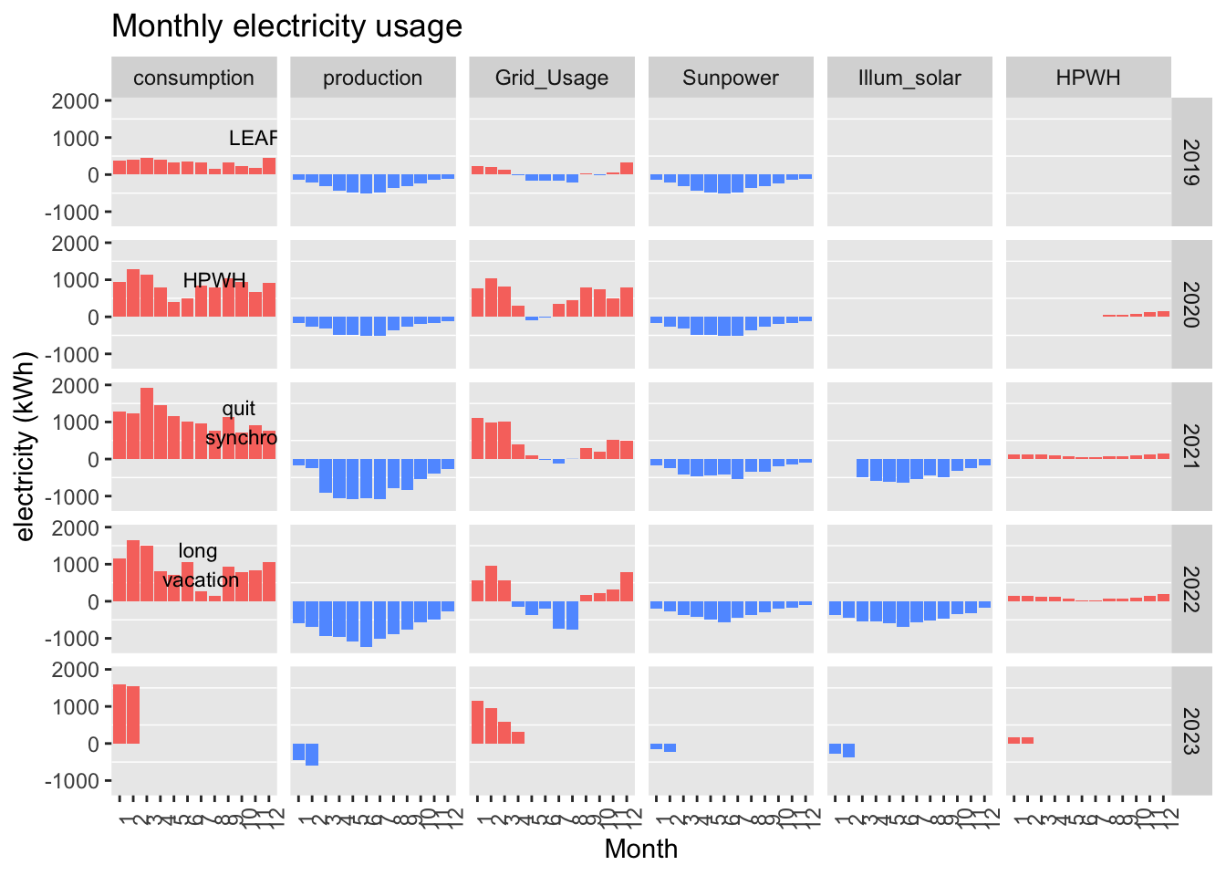
ggsave(file.path("Monthly_electricity_usage_summary.png"),height=8,width=11)Dual y-axis (see https://freyasystems.com/creating-a-dual-axis-plot-with-ggplot2/)
Keys are usage of sec_axis() in scale_y_continuous() and adjusting scale by multiplying (0.02) in sec_axis() and dividing data (0.02). Usually % HPWH is betweeen 5 and 20 % of monthly consumption.
# only `% water heat pump in consumption`
energy.all %>% ggplot(aes(x=month,y=`% HPWH in consumption`)) + geom_point() +   facet_grid(year~.)
## Warning: Removed 3 rows containing missing values (geom_point).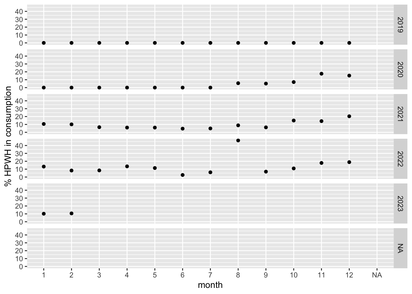
# Consumption and `% water heat pump in consumption` in one plot with dual axis
energy.all %>%
  pivot_longer(
  cols=c(consumption),
  values_to="kWh"
) %>% drop_na("kWh")  %>% drop_na("year.month2") %>% ggplot(aes(x=month,y=kWh)) + geom_bar(stat="identity") + geom_point(aes(x=month,y=`% HPWH in consumption`/0.02),color="green") +
  scale_y_continuous(
    sec.axis = sec_axis(~.* 0.02, name = "% HPWH in consumption")
  ) + facet_grid(year~.) + labs(title="electricity consumption and heat pump water heater usage",y="consumption (kWh)")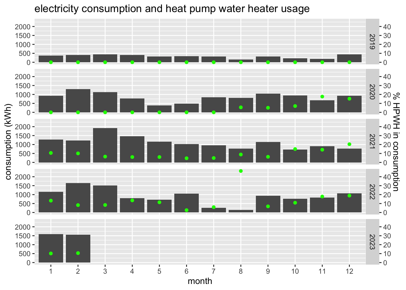
ggsave(file.path("HPWH_summary.png"),height=4,width=4*4/3)sessionInfo()## R version 3.6.2 (2019-12-12)
## Platform: x86_64-apple-darwin15.6.0 (64-bit)
## Running under: macOS 10.16
##
## Matrix products: default
## BLAS: /Library/Frameworks/R.framework/Versions/3.6/Resources/lib/libRblas.0.dylib
## LAPACK: /Library/Frameworks/R.framework/Versions/3.6/Resources/lib/libRlapack.dylib
##
## locale:
## [1] en_US.UTF-8/en_US.UTF-8/en_US.UTF-8/C/en_US.UTF-8/en_US.UTF-8
##
## attached base packages:
## [1] stats graphics grDevices utils datasets methods base
##
## other attached packages:
## [1] forcats_0.5.2 stringr_1.4.1 dplyr_1.0.10 purrr_0.3.5
## [5] readr_2.1.3 tidyr_1.2.1 tibble_3.1.8 ggplot2_3.3.6
## [9] tidyverse_1.3.2 lubridate_1.8.0
##
## loaded via a namespace (and not attached):
## [1] assertthat_0.2.1 digest_0.6.30 utf8_1.2.2
## [4] R6_2.5.1 cellranger_1.1.0 backports_1.4.1
## [7] reprex_2.0.2 evaluate_0.17 highr_0.9
## [10] httr_1.4.4 blogdown_1.13 pillar_1.8.1
## [13] rlang_1.0.6 googlesheets4_1.0.1 readxl_1.4.1
## [16] rstudioapi_0.14 jquerylib_0.1.4 rmarkdown_2.17
## [19] labeling_0.4.2 googledrive_2.0.0 bit_4.0.4
## [22] munsell_0.5.0 broom_1.0.1 compiler_3.6.2
## [25] modelr_0.1.9 xfun_0.34 systemfonts_0.3.2
## [28] pkgconfig_2.0.3 htmltools_0.5.3 tidyselect_1.2.0
## [31] bookdown_0.29 fansi_1.0.3 crayon_1.5.2
## [34] tzdb_0.3.0 dbplyr_2.2.1 withr_2.5.0
## [37] grid_3.6.2 jsonlite_1.8.3 gtable_0.3.1
## [40] lifecycle_1.0.3 DBI_1.1.3 magrittr_2.0.3
## [43] scales_1.2.1 cli_3.4.1 stringi_1.7.8
## [46] vroom_1.6.0 cachem_1.0.6 farver_2.1.1
## [49] fs_1.5.2 xml2_1.3.3 bslib_0.4.0
## [52] ellipsis_0.3.2 generics_0.1.3 vctrs_0.5.0
## [55] tools_3.6.2 bit64_4.0.5 glue_1.6.2
## [58] hms_1.1.2 parallel_3.6.2 fastmap_1.1.0
## [61] yaml_2.3.6 colorspace_2.0-3 gargle_1.2.1
## [64] rvest_1.0.3 knitr_1.40 haven_2.5.1
## [67] sass_0.4.2